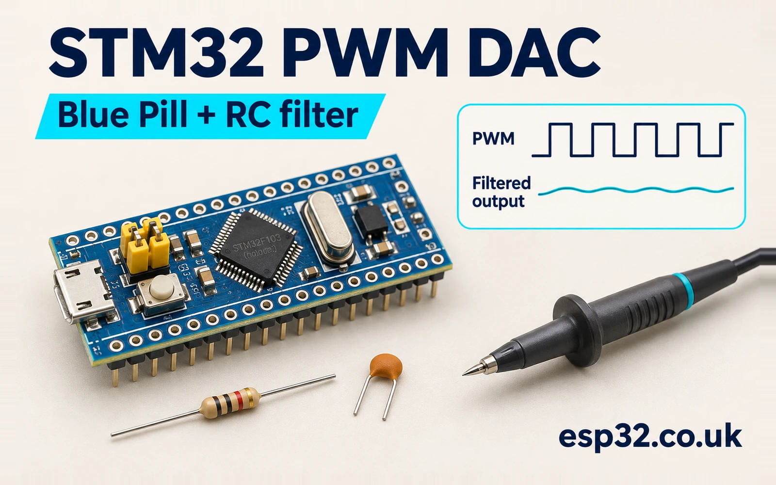
The STM32F103C8PriceAliExpress price Blue PillPriceAliExpress price can produce an adjustable analogue voltage using a timer output and two passive components. In this esp32.co.uk/ guide, TIM3 drives PA6 at 20 kHz. A series resistorPrice and a capacitor to ground average the pulse train. The project sets the desired voltage in millivolts, and an oscilloscope or meter verifies what the circuit actually delivers.
Use this approach for a slow, high-impedance setpoint or an analogue-output experiment. The timer determines the duty-cycle increment. The filter, load and GPIO supply determine how closely the physical output follows a request. The lab calculates those effects separately and gives you a repeatable method to measure them. Start with 10 kΩ and 100 nF, then compare a larger capacitor when you need less ripple.
Decide what the analogue output must do
Write down three numbers before selecting components. Set the output range, the maximum acceptable carrier ripple and the time allowed for a new setpoint to settle. A fourth quantity, load impedance, is just as important once the node connects to anything beyond a meter. For instance, a slow comparator reference can tolerate several milliseconds of response time. An output intended to reproduce a fast waveform has a different bandwidth and ripple budget.
The Blue PillAliExpress price’s STM32F103C8 provides timer PWM and ADC inputs. This device does not include a DAC peripheral. The analogue output in this lab is the voltage across an external capacitor. The GPIO still switches between its low and high levels. The filter reduces the alternating component, and the average depends on the fraction of the period spent high. The TI discussion of PWM-derived analogue control describes the same ripple and settling trade-off. ST STM32F103C8 datasheet · TI PWM and DAC comparison
| Quantity | Meaning in this lab |
|---|---|
| Requested voltage | Firmware command expressed as an integer number of millivolts |
| Average output | Mean of the periodic voltage after settling |
| Ripple | Difference between the maximum and minimum within a carrier period |
| Settling time | Time for the chosen envelope or measured quantity to approach its new value |
| Static accuracy | Difference between the commanded voltage and the measured settled average |
| Load impedance | Resistance and capacitance connected to the filtered node |
Keep those quantities separate when discussing resolution. An increment of one timer count changes the nominal unloaded average by less than one millivolt in this setup. The instantaneous voltage can still move by tens of millivolts within a carrier cycle. A digital multimeter may display a stable average while a threshold detector attached to the same node reacts to the ripple. An application specification should say whether it cares about the average, the instantaneous voltage or a sampled value at a particular phase.
For a capstone bench exercise, try the same command with two capacitors and then with a known load. Use the first comparison to measure the ripple and settling trade-off. Use the second to see why the same duty cycle can produce a different average. That sequence ties a working timer configuration to an electrical model without relying on a display library or a separate analogue peripheral.
Wire the RC output
Use a genuine STM32F103C8 board, an SWD probe, one resistor and one capacitor. Connect PA6 to one end of a 10 kΩ resistor. The other end is the filtered output. Connect 100 nF from that output node to ground. Connect the meter or oscilloscope to the filtered node and the same board ground. The resistor belongs in series with the GPIO, and the capacitor belongs across the output and ground. The two probe points should be easy to reach independently.
| Connection | Bench setup |
|---|---|
| PA6 | TIM3 channel 1 with default pin mapping |
| Series resistor | 10 kΩ from PA6 to the analogue node |
| Capacitor | 100 nF from the analogue node to GND |
| Raw PWM probe | PA6 referenced to board GND |
| Analogue probe | Capacitor node referenced to board GND |
| SWD | Normal debugger pins, separate from PA6 |
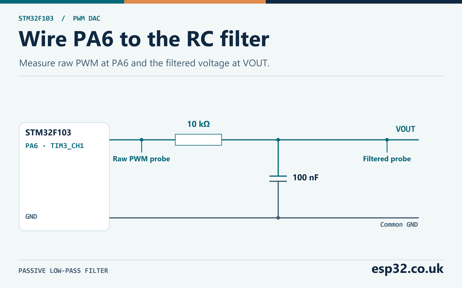
Start with a high-impedance instrument. A meter with 10 MΩ input resistance makes a much lighter load than a 100 kΩ circuit. An oscilloscope probe can add both resistance and capacitance, and its effective resistance depends on the probe setting and the instrument’s termination. Check the probe documentation. A 50 Ω termination would be a very heavy load for this network. Measure at the resistor-capacitor junction, where the expected signal is a mostly steady voltage with a smaller ripple. Blue Pill pinout guide
Keep the return path short and connect the probe ground to the same ground used by the capacitor. A long ground lead can show ringing that is partly a measurement artefact. Save one trace at the GPIO and one at the capacitor node. If you use two scope channels, check that both probes have the expected attenuation. A large mismatch between the reported GPIO high and the board supply can be a probe configuration issue before it is a circuit issue.
At the start of a rising edge with the capacitor near ground, the series resistor limits current to about 3.3 V divided by 10 kΩ, or 0.33 mA in the ideal calculation. That current decreases as the capacitor charges. A falling edge lets the GPIO sink current through the resistor. Avoid connecting a large capacitor directly to PA6. The series element is part of the intended circuit and limits the GPIO load during transients.
Measure the component values if you want to compare the trace closely with a prediction. A capacitor’s effective value can differ from its marking because of tolerance, temperature and DC bias, depending on its construction. A 10% lower effective capacitance produces a smaller time constant, a faster step response and more carrier ripple. Record the actual component type and measured value when evaluating a proposed tolerance. A circuit that meets the target with nominal parts may have less margin across a batch.
Before flashing, check the passive wiring with power off. Measure continuity from PA6 to the resistor, then confirm that the capacitor node has no direct short to ground. A resistance reading across the capacitor may change as the instrument charges it. After applying power, request zero duty first and confirm that the output returns near ground. Then request full duty and record both the raw pin voltage and the filtered node. The difference between those readings exposes static loading or leakage before you introduce any ripple.
Set TIM3 to a 20 kHz carrier
Configure the Blue Pill for a 72 MHz system clock with AHB divide by one and APB1 divide by two. The example fixture uses a nominal 8 MHz HSE crystal and a PLL multiplier of nine. With a divided APB1 clock, TIM3 receives twice PCLK1 on this STM32F1, giving 72 MHz with PCLK1 at 36 MHz. A board with a different external oscillator requires the corresponding Cube configuration. The module checks the expected nominal clock settings and does not measure the oscillator directly. ST RM0008 reference manual · STM32CubeMX setup guide
For an edge-aligned up-counter, the period contains ARR plus one counts. The prescaler divides the timer input by PSC plus one. At PSC zero and ARR 3599, the carrier is 72,000,000 divided by 3600, or 20,000 Hz. Each period lasts 50 µs. In active-high PWM mode 1, the output is high while the counter is below the active compare value. Half duty requires CCR1 equal to 1800, with 25 µs high and 25 µs low. STM32 timer and PWM guide
| Requested ideal output | Duty at a 3.3 V high | CCR1 | High time |
|---|---|---|---|
| 0 V | 0% | 0 | 0 µs |
| 0.825 V | 25% | 900 | 12.5 µs |
| 1.650 V | 50% | 1800 | 25.0 µs |
| 2.475 V | 75% | 2700 | 37.5 µs |
| 3.300 V | 100% | 3600 | Entire period |
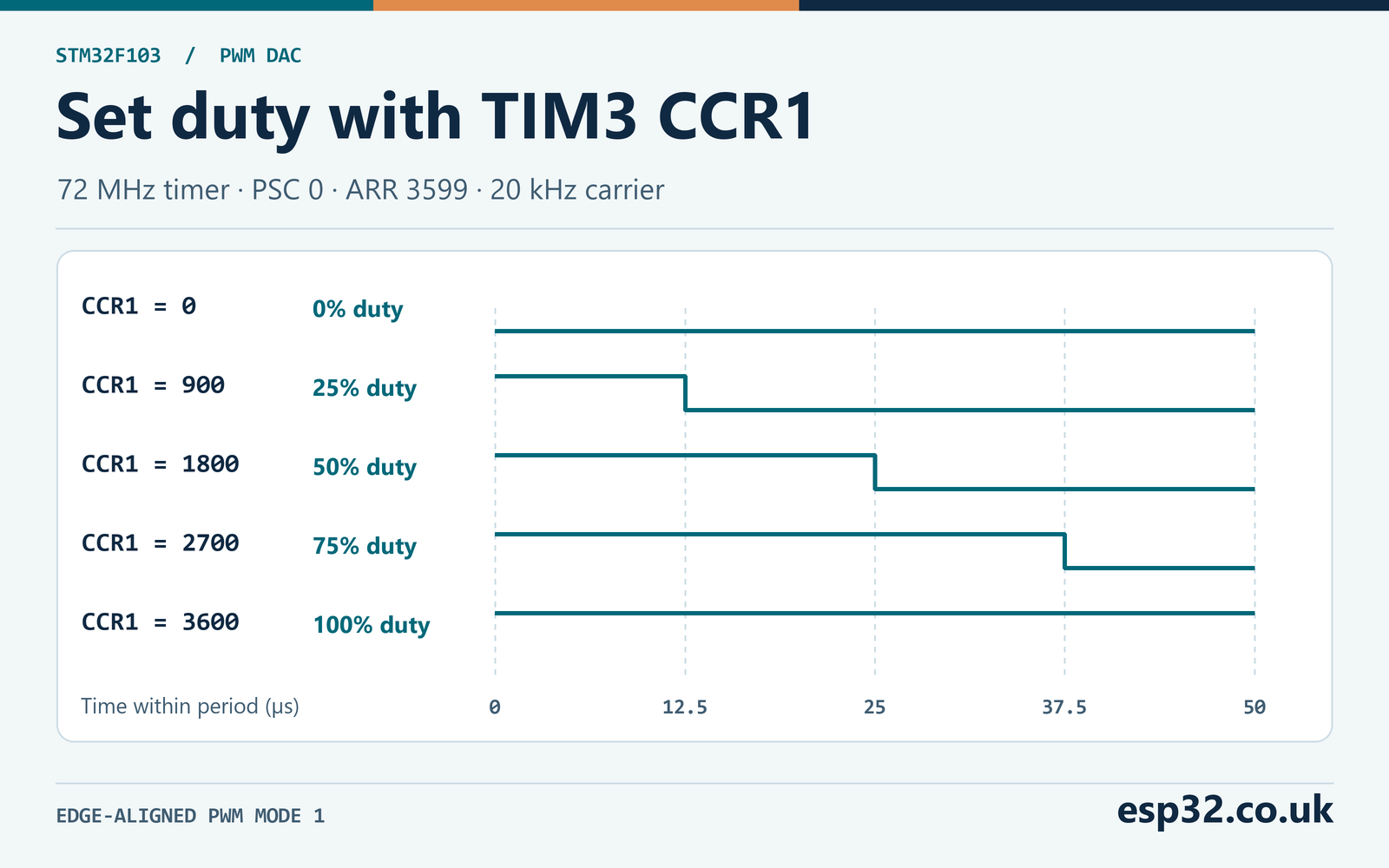
CCR1 equal to zero keeps the output low. CCR1 equal to 3600 keeps it high because the counter never reaches 3600. This is valid for the chosen 16-bit compare register and ARR setting. A design with ARR already at 65535 cannot represent ARR plus one in that 16-bit register. When reusing the method on another timer, check the endpoint behavior and compare width before assuming the same code can produce a constant high.
The module enables compare preload. A write to CCR1 is staged and becomes active at a timer update, so changing the voltage command during a carrier period does not reshape that period halfway through. If several writes occur before one update, the last staged value takes effect. The expected software-to-waveform latency is up to about one carrier period when writes are infrequent. The RC response starts after the new waveform takes effect and is usually much slower in this design. ST STM32F1 timer HAL v1.1.10
There are 3600 equal duty intervals and 3601 commandable compare values including both endpoints. One interval corresponds to 3.3 V divided by 3600, approximately 0.917 mV of unloaded average. A nearest-count mapping adds up to about 0.458 mV of ideal rounding error when the requested voltage is represented exactly. That calculation excludes the integer-millivolt API quantization, the supply uncertainty, the load and ripple. A higher PWM carrier would generally reduce ripple for the same filter, but at a fixed timer input it leaves fewer counts per period.
Check the carrier first when the waveform is wrong. A period of 100 µs instead of 50 µs suggests the timer is running at 36 MHz with the same divider settings, or that the programmed period is twice what you intended. Read the RCC prescaler, PSC and ARR and verify which timer actually drives PA6. A correctly averaged voltage at half duty does not prove the carrier frequency is correct. The same average can coexist with much larger ripple if the period is longer.
At 20 kHz, a scope that displays just a few periods gives a useful timing check. At a small duty you may need to zoom far enough to distinguish a narrow pulse from an edge or a display artefact. To verify preload, temporarily request two visibly different intermediate values at a known interval. Trigger on the change in pulse width and inspect the last old period and first new period. Each should have its intended width. A phase change or truncated pulse suggests that the update path or another writer changed the timer configuration.
Calculate ripple and step response
With a high-impedance load and an ideal GPIO, the RC time constant is R times C. At 10 kΩ and 100 nF it is 1 ms. The first-order corner frequency is 1 divided by two pi times the time constant, about 159 Hz. The carrier is well above that corner, so the capacitor voltage charges a little during each high interval and discharges a little during each low interval. It does not become perfectly flat.
The time average is approximately the low level plus duty times the difference between the high and low levels. In the ideal unloaded linear circuit it is exactly that value in periodic steady state. Over a full period the capacitor’s net change in voltage is zero. The average resistor current is therefore zero and the average voltage drop across the resistor is zero. This provides a useful way to reason about the mean without mistaking it for either peak of the ripple.
For an exact unloaded ripple calculation, let a be exp of minus the high time divided by the time constant, and b be exp of minus the low time divided by the time constant. With ideal levels 0 V and Vhigh, the steady-state peak is Vhigh times (1 minus a) divided by (1 minus a times b). The trough is b times the peak. The difference gives the peak-to-peak ripple. The result follows by charging from the trough during the high interval, then discharging from the peak during the low interval and returning to the same trough.
At half duty, a and b are both exp of minus 25 µs divided by 1 ms. The peak-to-peak ripple simplifies to Vhigh times (1 minus a) divided by (1 plus a). With 3.3 V this gives about 41.25 mV peak to peak. The corresponding trough and peak are about 1.6294 V and 1.6706 V. The arithmetic mean of those two is 1.65 V at half duty. At other duties, use the time average rather than assuming the mean of the extrema equals it.
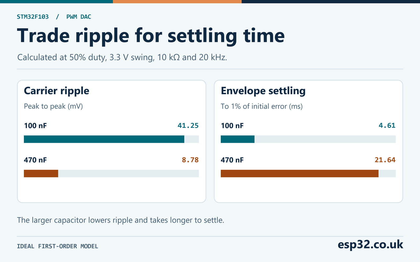
For a step command, the difference from the new periodic waveform decays exponentially in the ideal linear model. That difference reaches 1% of its initial value after about 4.605 time constants. The output continues to ripple around the new average. At half duty the 100 nF circuit still has roughly 20.6 mV excursion on each side once settled, so a requirement to stay within 1% of a 1.65 V step cannot be satisfied by waiting alone. Reduce ripple or define a phase-aware or averaged measurement.
| Capacitor with 10 kΩ | Time constant | Corner frequency | Half-duty ripple at 20 kHz | Time to 1% of initial error |
|---|---|---|---|---|
| 47 nF | 0.47 ms | 339 Hz | 87.75 mV p-p | 2.16 ms |
| 100 nF | 1.00 ms | 159 Hz | 41.25 mV p-p | 4.61 ms |
| 470 nF | 4.70 ms | 33.9 Hz | 8.78 mV p-p | 21.64 ms |
| 1 µF | 10.00 ms | 15.9 Hz | 4.12 mV p-p | 46.05 ms |
The table uses ideal components and an unloaded node. The half-duty case is a useful design check because a single-pole filter driven by this ideal pulse train has its largest steady-state ripple there. At zero and full duty the pin holds a constant level and there is no carrier ripple after settling. For an intermediate command close to an endpoint, inspect the short high or low time at PA6 as well as the output. Real edge duration and GPIO impedance can matter when the requested pulse is only a few timer ticks wide.
Suppose the target is at most 10 mV peak to peak at half duty and a roughly 25 ms envelope settling budget. The 470 nF option predicts 8.78 mV and about 21.64 ms before tolerances. This leaves only modest margin for capacitance, carrier frequency, loading and measurement error. If the effective capacitance falls by 20%, the predicted ripple rises to about 10.97 mV. Choose parts or requirements with that margin in view. A test at nominal voltage with one sample establishes a baseline for tolerance testing. TI discussion of PWM filter settling
The filter corner is also a signal-bandwidth limit. If you update the duty at a high rate, the node cannot follow arbitrary fast steps just because the timer accepts them. A commanded sine wave well below the corner is easier to reproduce than one near or above it. For a changing setpoint, decide whether amplitude attenuation and phase lag are acceptable. The simple RC lab targets slow control voltages and makes the filtering effects easy to observe.
You can size the time constant directly from a ripple target at half duty. In this ideal model, peak-to-peak ripple equals the high-to-low swing times the hyperbolic tangent of the period divided by four time constants. For a 3.3 V swing and 10 mV allowable ripple, solve for a time constant of about 4.125 ms or more at 20 kHz. With 10 kΩ, the nominal minimum capacitance is therefore about 413 nF before tolerances. That result explains why 470 nF is a useful comparison value. The step-response constraint independently puts an upper limit on the time constant.
You can also measure the time constant without resolving millivolts of ripple. Change the command from constant low to constant high and time how long the node takes to reach roughly 63.2% of its final voltage. There is no steady carrier ripple at either endpoint. The measurement includes the timer’s update delay unless you trigger on the GPIO transition itself. Once you have measured the effective time constant, reuse it in the ripple calculation and compare against the half-duty trace. This helps separate a component tolerance from a carrier or probing problem.
Account for the connected load
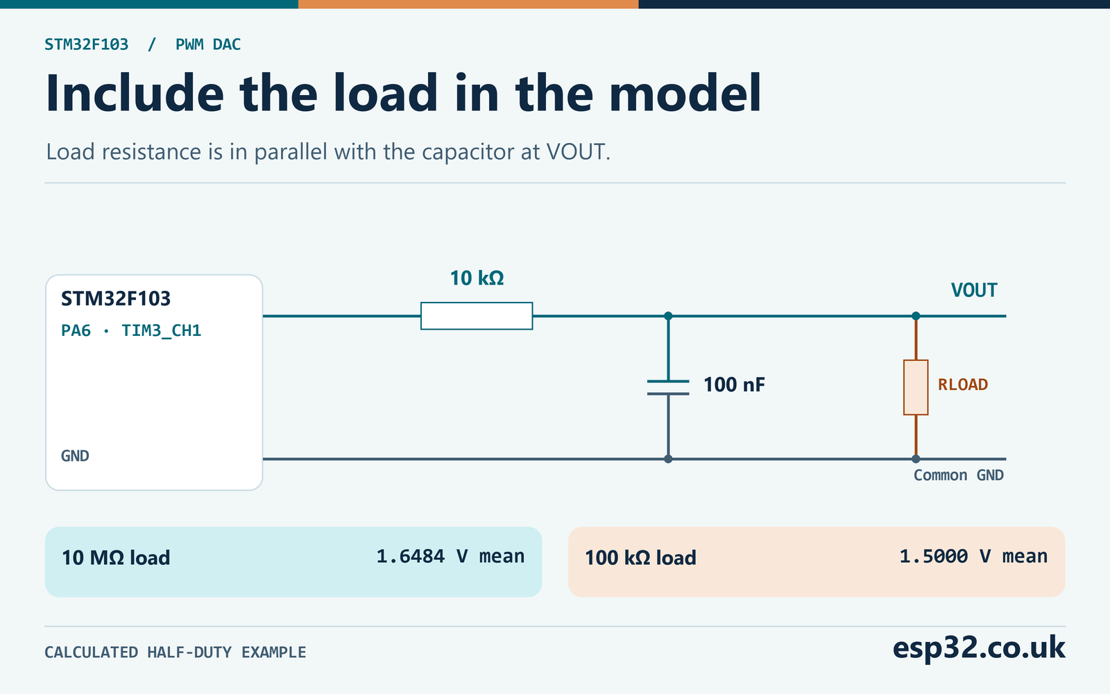
A resistor from the filtered node to ground forms a divider with the 10 kΩ series resistor. In steady state the ideal average is multiplied by Rload divided by the sum of Rload and Rseries. For example, 100 kΩ gives a gain of 0.9091 and a nominal half-duty output of 1.500 V. A 1 MΩ load gives about 1.6337 V and a 10 MΩ load about 1.6484 V. At the same time the capacitor sees the parallel combination of the series resistor and load for its time constant. The load therefore changes both the average and the response.
| Load to ground | Ideal DC gain | Mean at 50% duty |
|---|---|---|
| Open circuit | 1.0000 | 1.6500 V |
| 10 MΩ | 0.9990 | 1.6484 V |
| 1 MΩ | 0.9901 | 1.6337 V |
| 100 kΩ | 0.9091 | 1.5000 V |
| 10 kΩ | 0.5000 | 0.8250 V |
If a load needs more current, consider a suitable high-input-impedance buffer after the RC network. Check the amplifier’s supply range, input common-mode limits, output swing and stability with the actual load. A rail-to-rail label alone does not specify performance at the rail for every load. For the passive bench start with a meter, then add a known resistor and verify the divider prediction. That experiment is simpler than adjusting calibration constants to hide loading.
If you connect an ADC input, the load can vary during sampling. The input capacitance and sample switch can draw charge from the node. A longer acquisition time may help. Measure whether the ADC result or node changes when sampling starts, and use the exact F103 ADC input requirements when designing a measurement path. Keep the node within the ADC’s input range and use a common reference. If the sampling rate and PWM carrier are related, repeated samples can land at a similar phase and retain a ripple-dependent offset. STM32 ADC, calibration and DMA guide
The loaded time constant follows from replacing the GPIO source by its ideal zero-impedance equivalent when calculating the resistance seen by the capacitor. The load and the series resistor then both lead to ground. With 100 kΩ and 10 kΩ their parallel value is about 9.09 kΩ. With 100 nF that gives about 0.909 ms. Use the smaller time constant and the divider-scaled high level together when modelling ripple. Plugging the loaded average into the unloaded time response would mix two different circuits.
If a digital reader samples at exactly 1 kHz, there are twenty 20 kHz carrier periods between samples. In an ideal phase-locked example it can repeatedly read the same point on the ripple. Averaging those samples leaves the phase bias in place. Averaging over a measured whole number of carrier periods, sampling at multiple known phases or applying enough analogue attenuation changes that result. Check timing in the actual application before treating a stable digital reading as the mean.
Add the PWM DAC module to CubeF1
Create an STM32F103C8 project with Serial Wire debug and the 72 MHz clock tree described above. Include the CubeF1 TIM, GPIO and RCC HAL modules and their matching sources. Leave PA6 and TIM3 available for this module, which configures them and owns the timer. Other channels on TIM3 share the same time base. They may need a different timer if another part of your project expects a different carrier frequency. Keep the HAL tick running for the example loop.
The module starts PA6 as a low GPIO output, then configures the timer with a zero compare and starts PWM before handing the pin to its alternate function. The initial state is low during this setup sequence. The pin can still be high impedance before firmware starts, so design a separate defined startup state if the attached circuit requires one through reset. The example is foreground code. Give one caller ownership of the output to keep conflicting commands from racing.
#ifndef PWM_DAC_H
#define PWM_DAC_H
#include "stm32f1xx_hal.h"

enum { PWM_DAC_COUNTS = 3600 };

/* TIM3 channel 1 on PA6, default remap. Call after the clock setup. */
HAL_StatusTypeDef PwmDac_Start(void);

/* Set the requested output in mV. rail_mv is the measured unloaded high level. */
HAL_StatusTypeDef PwmDac_SetMillivolts(uint16_t requested_mv, uint16_t rail_mv);

#endif
#include "pwm_dac.h"
static TIM_HandleTypeDef timer;
static uint8_t started;
HAL_StatusTypeDef PwmDac_Start(void)
{
if (HAL_RCC_GetPCLK1Freq() != 36000000U ||
(RCC->CFGR & RCC_CFGR_PPRE1) != RCC_CFGR_PPRE1_DIV2) {
return HAL_ERROR;
}
if (started) {
return HAL_OK;
}
__HAL_RCC_AFIO_CLK_ENABLE();
if (AFIO->MAPR & AFIO_MAPR_TIM3_REMAP) {
return HAL_ERROR;
}
__HAL_RCC_TIM3_CLK_ENABLE();
__HAL_RCC_GPIOA_CLK_ENABLE();
__HAL_RCC_TIM3_FORCE_RESET();
__HAL_RCC_TIM3_RELEASE_RESET();
GPIO_InitTypeDef pin = {
.Pin = GPIO_PIN_6, .Mode = GPIO_MODE_OUTPUT_PP,
.Pull = GPIO_NOPULL, .Speed = GPIO_SPEED_FREQ_LOW
};
HAL_GPIO_WritePin(GPIOA, GPIO_PIN_6, GPIO_PIN_RESET);
HAL_GPIO_Init(GPIOA, &pin);
timer.Instance = TIM3;
timer.Init.Prescaler = 0U;
timer.Init.CounterMode = TIM_COUNTERMODE_UP;
timer.Init.Period = PWM_DAC_COUNTS - 1U;
timer.Init.ClockDivision = TIM_CLOCKDIVISION_DIV1;
timer.Init.AutoReloadPreload = TIM_AUTORELOAD_PRELOAD_ENABLE;
const TIM_OC_InitTypeDef channel = {
.OCMode = TIM_OCMODE_PWM1, .Pulse = 0U,
.OCPolarity = TIM_OCPOLARITY_HIGH, .OCFastMode = TIM_OCFAST_DISABLE
};
if (HAL_TIM_PWM_Init(&timer) != HAL_OK ||
HAL_TIM_PWM_ConfigChannel(&timer, &channel, TIM_CHANNEL_1) != HAL_OK) {
return HAL_ERROR;
}
SET_BIT(TIM3->CCMR1, TIM_CCMR1_OC1PE);
TIM3->EGR = TIM_EGR_UG;
if (HAL_TIM_PWM_Start(&timer, TIM_CHANNEL_1) != HAL_OK) {
return HAL_ERROR;
}
pin.Mode = GPIO_MODE_AF_PP;
HAL_GPIO_Init(GPIOA, &pin);
started = 1U;
return HAL_OK;
}
HAL_StatusTypeDef PwmDac_SetMillivolts(uint16_t requested_mv, uint16_t rail_mv)
{
if (!started || !rail_mv || requested_mv > rail_mv) {
return HAL_ERROR;
}
uint32_t compare = ((uint32_t)requested_mv * PWM_DAC_COUNTS + rail_mv / 2U) / rail_mv;
__HAL_TIM_SET_COMPARE(&timer, TIM_CHANNEL_1, compare);
return HAL_OK;
}Declare the watch variables in a generated user region. Place the remaining statements after clock initialization, then update the request in the foreground loop. The nominal 3300 mV high level is a starting point. For an unloaded estimate measure PA6 at full duty and use the measured high level in millivolts. This single-parameter mapping assumes the low level is close to zero. If you need to compensate both endpoints, measure both under the intended load and fit a separate two-point mapping.
#include "pwm_dac.h"
volatile uint16_t requested_mv = 1650;
volatile HAL_StatusTypeDef dac_status;

/* After HAL_Init and system clock configuration. */
dac_status = PwmDac_Start();
if (dac_status != HAL_OK) {
    for (;;) { __NOP(); }
}
for (;;) {
    dac_status = PwmDac_SetMillivolts(requested_mv, 3300U);
    HAL_Delay(20U);
}
The function returns an error when it has not started, the rail value is zero or the request exceeds the rail. A rejected setpoint leaves the prior compare value in place. Use that behavior intentionally in your application. If a bad command should instead drive the output to zero, apply that policy in the caller and confirm the safe voltage at the connected circuit. The 20 ms delay here is a convenient interval for the foreground loop, and the timer continues running between calls. It is independent of the 50 µs carrier period and the analogue settling time.
Verify voltage, ripple and settling
Start at half duty and measure at PA6. You should see about 50 µs between rising edges and about 25 µs high. Move the probe to the capacitor node. On a DC-coupled trace confirm that the mean is near the predicted voltage. Then zoom the vertical scale or use AC coupling to see the ripple. Use DC coupling when measuring absolute voltage or a slow step, since AC coupling removes the DC level and can distort slow changes. Record the actual probe impedance and the bandwidth setting.
Capture several consecutive carrier cycles and estimate the peak-to-peak ripple from the repeating waveform. A scope’s automatic peak-to-peak measurement can include occasional noise spikes if you give it a long acquisition. Compare the repeating excursion with the wider noise floor. If the measured ripple is larger than predicted, verify the capacitor value and carrier before changing the firmware. Measure supply noise too. The filtered output can reflect changes in the GPIO’s high level.
For a settling measurement, step from zero to half duty and trigger on the first carrier activity or the analogue rise. In the 100 nF circuit the ideal envelope should traverse about 63% of the step after 1 ms and approach its new periodic waveform over several milliseconds. Use the same definition when comparing with the 470 nF circuit. If you average over carrier cycles, record the averaging window, because it contributes its own delay. If you sample the same phase across periods, compare those samples with their final phase value.
| Observation | What to check |
|---|---|
| PA6 is quiet and initialization failed | Clock tree, APB1 divider and TIM3 remap |
| Period correct and duty wrong | CCR1, requested millivolts and rail parameter |
| Mean too low with a correct raw waveform | Load, probe termination and actual high level |
| Ripple larger than expected | RC values, carrier period, measurement and ground path |
| Slow step with acceptable ripple | Time constant and update-to-measurement timing |
| Near-rail values miss the target | Actual high and low levels, loading and settling |
| Meter and ADC disagree | Acquisition, reference, sample phase and averaging |
After the first tests, sweep a handful of setpoints from zero to full duty. Use the same load and wait long enough for the chosen filter after each change. Record the requested value, actual compare, GPIO high and low, mean output and ripple. A consistent gain error suggests a rail or loading difference. A constant offset near mid-scale suggests an endpoint or measurement reference issue. A discrepancy concentrated near an endpoint can be a pulse-width or output swing limit. The sweep is more informative than calibrating at half duty alone.
To test load sensitivity, measure the settled half-duty voltage with just the probe, then add the 100 kΩ load. Compare the observed change with the divider prediction and the new effective time constant. Remove the load and repeat the original measurement. This catches cases where a probe setting or a cable change is responsible for the difference. If you later add a buffer, repeat the same test at its output and verify both the mean and stability.
For two-point calibration, use the measured minimum and maximum at the final load. Subtract the measured low level from the target and divide by the measured span to get duty, then convert duty to a compare value. Reject or clamp requests outside the measured range according to application policy. For example, if the endpoints are 5 mV and 3005 mV, a request for 1505 mV is halfway through the measured span and maps to 1800. The calibration can correct a static slope and offset. It leaves the carrier ripple, settling behavior and changes in loading visible, so repeat the sweep after calibration.
Choose when to use a dedicated DAC
A passive PWM output is useful when the load is light, the setpoint moves slowly and the remaining ripple is acceptable. It uses one timer channel and two components. The analogue accuracy depends on the GPIO supply, output levels, filter components and attached circuit. If you need fast settling and much lower ripple simultaneously, evaluate a dedicated DAC or a higher-order filter with a properly specified buffer. Include update rate, accuracy, output impedance and start-up behavior in that comparison.
Changing only the PWM frequency is one design lever. For example, doubling the carrier to 40 kHz at a 72 MHz timer input reduces the period to 1800 counts and doubles the nominal size of one duty increment. For a 1 ms time constant it approximately halves the half-duty ripple. The simple module fixes the carrier at 20 kHz. Any change should be followed by a fresh calculation of compare values, the end conditions and the ripple budget, then a repeat of the bench sweep.
If the project changes clock settings during operation, treat the analogue output as part of that transition. A timer that slows down produces longer high and low intervals, and the ripple can rise even if the duty ratio remains unchanged. A timer that stops can leave the pin at one level while the capacitor moves toward that level. The setup guard in this lab checks the clock before starting, and the setter assumes that the clock and pin ownership remain stable. Define the output’s expected behavior during low-power entry or reconfiguration separately if it drives another circuit.
A useful final comparison records the intended filter, the measured effective time constant and the loading condition together. For instance, a design may meet its output average with a 10 MΩ probe yet fail after adding a 100 kΩ destination. Keep those traces under separate labels. If you later change to a buffered output or a dedicated DAC, reuse the same sweep and step criteria so the comparison reflects how the application uses the output.
Keep the clock configuration and scope traces with the final circuit. A raw waveform confirms the digital configuration. A ripple trace and step capture show what the filter does. A loaded sweep shows what the attached circuit receives. Taken together, those measurements let you decide whether the output meets the original requirements and give you a baseline for changing the timer, capacitor or load in the next design.
Repeat the ripple check near the intended operating point after assembly. The worst-case half-duty calculation is useful for a full-range design, but a system that uses only a narrow duty range may have a different practical ripple budget. Record the actual range rather than assuming the full-scale result describes every operating condition.