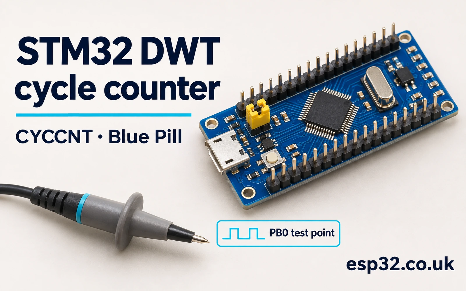
The STM32PriceAliExpress price DWT cycle counter measures short stretches of firmware in processor cycles. In this esp32.co.uk/ guide you will enable DWT->CYCCNT on an STM32F103C8PriceAliExpress price Blue PillPriceAliExpress price, take two snapshots, and measure an empty call, a block of 32 NOP instructions and two GPIO implementations. The complete STM32Cube HAL example records minimum, maximum and total cycles over 64 trials. A scope on PB0 gives you an independent way to see the resulting output pulses.
Start with the empty measurement and the NOP block. They tell you whether the counter runs and how much work the measurement itself adds. Then compare the GPIO paths in the same firmware image and use the active core clock to convert the numbers to time. The benchmark measures CPU-side execution, including stalls or interrupts within the bracket. The scope measures voltage at the pin, which answers a related electrical question.
What the STM32 DWT cycle counter measures
DWT stands for Data Watchpoint and Trace. On a Cortex-M3 implementation that provides the cycle counter, CYCCNT is a 32-bit register that increments on processor clock cycles while enabled and running. The register belongs to the processor’s debug and trace facilities. It is accessed through the CMSIS core definitions, so the example needs no spare STM32 timer and no interrupt handler to increment a software variable. The firmware reads the local counter directly. Serial Wire Viewer and an SWO wire are unnecessary for those reads. Arm Cortex-M3 Technical Reference Manual · Arm CMSIS Cortex-M3 header
Imagine comparing two ways to send a single GPIO update. A millisecond tick is too coarse for this job. A hardware timer can measure short intervals, but it has its own clock and may already be assigned to a capture, PWM or scheduling task. CYCCNT gives you the processor’s cycle count across two points in the code. Use those cycles to compare instruction sequences under the same clock and build settings. If the question is when an external input changed or when a pin reached a logic level, use an input capture peripheral or an instrument on the wire. STM32 timer and input capture guide
A cycle is one period of the clock, while an instruction can take different numbers of cycles depending on its operation and where data and instructions come from. The core can wait for a bus response or Flash fetch. Branches and exception entry also affect elapsed cycles. For this reason, reading a cycle counter around a workload answers how long that executed path took under its current conditions. Counting the source statements, or counting the instructions in a listing, answers a different question.
| Measurement question | Instrument or timebase | What the number describes |
|---|---|---|
| How long did a short C function take? | DWT CYCCNT | Processor cycles within the measurement bracket |
| Did the output pulse meet the circuit’s requirement? | Oscilloscope on PB0 | Voltage transitions and pulse width at the test point |
| When did an external edge arrive? | Timer input capture | Hardware timestamp in timer ticks |
| How much real time elapsed across a low-power interval? | A suitable RTC or external instrument | Time on a clock that remains active in that mode |
The target here is the STM32F103C8 with an Arm Cortex-M3 core. Other STM32 families have different processor and debug implementations. Check the exact core’s documentation and device header before porting the code. A header that exposes a type or register address is only one piece of evidence. Confirm that the feature is implemented, accessible in the privilege mode you use, and ticking on the physical target. The F103 device datasheet, programming manual and core header give you those starting points. ST STM32F103C8 datasheet · ST Cortex-M3 programming manual PM0056
Set up the Blue Pill and scope
Use a genuine STM32F103C8 board, a working SWD programmer and a fresh CubeF1 project. In CubeMX select the exact device, retain Serial Wire debug and configure PB0 as a GPIO output. Set it initially low, with push-pull mode and no pull resistor. The lab uses the high GPIO speed setting. Use the same setting for both implementations and leave PB0 assigned to this lab only. A dedicated GPIO test point keeps the comparison independent of board-specific LED polarity, LED loading and pin assignments. Blue Pill pinout guide · STM32 GPIO and HAL guide
| Setting or connection | Lab configuration |
|---|---|
| MCU and HAL project | STM32F103C8, CubeF1 with STM32Cube HAL |
| Debug pins | PA13 SWDIO and PA14 SWCLK |
| Test output | PB0, push-pull, initially low, no pull |
| GPIO clock | Enable GPIOB on APB2 before configuring PB0 |
| Probe | Scope tip on PB0 and ground at nearby board GND |
| Clock for conversion | HCLK after system clock setup |
| Timebase for the rest of HAL | Keep the project’s normal HAL tick |
The bench can run with the default 8 MHz HSI configuration or a valid CubeMX clock tree at 72 MHz. Check the clock diagram and actual configuration before assuming the maximum rate. At 72 MHz the core uses a different Flash latency setup from the 8 MHz case. A project intended to compare the effect of changing HCLK should record the system clock source, prescalers and Flash configuration. A result that changes between these runs can reflect several real differences in the platform. CubeMX and CubeIDE setup · ST RM0008 reference manual
Connect the scope ground to board ground before probing PB0. A short ground spring and a probe with suitable bandwidth make a narrow pulse easier to see. Use single-shot acquisition or persistence and trigger on a rising edge. The code executes the test once at boot and then leaves the results available to inspect. Arm the scope before running or resetting the program. Several bursts follow closely, so capture a wider time span first and zoom in after you find the pulses. ST-Link wiring guide
If the scope misses the short pulse, check probe attenuation, sample rate, trigger level and whether you captured the first run. To validate the connection itself, build a separate slow GPIO toggle or use the GPIO tutorial’s blink loop with PB0 as the output. Put the original benchmark back before collecting timings. Adding delay calls between the two GPIO writes produces a visible test pulse and also changes the program being measured, so keep that wiring check out of the reported comparison.
If you test a different HCLK, keep track of PCLK2 as well. For example, a configuration with HCLK at 72 MHz and APB2 divided by two puts PCLK2 at 36 MHz. The nanoseconds conversion still uses 72 MHz. GPIO access crosses into the APB2 domain, so a change to that divider can change the number of core cycles needed for the same register sequence. The timer clock multiplier that can apply to an APB timer is irrelevant to this conversion. For a clean HAL-versus-BSRR comparison, measure both paths before touching the clock tree.
You can cross-check the configured HCLK with a long reference interval if the system appears to be running at the wrong rate. One bench method is to configure a timer output with a known period and measure that period on the scope. Derive the expected period from the actual timer input clock, prescaler and auto-reload. If the observed period is twice what you expected, work back through the clock source and bus dividers. This is also useful when the board crystal marking and the oscillator constant used by the firmware disagree. The cycle counts can still be useful for comparing two code paths even before the conversion to physical time has been confirmed.
Enable CYCCNT and check that it moves
Set CoreDebug->DEMCR.TRCENA first. In C the CMSIS field mask is CoreDebug_DEMCR_TRCENA_Msk, and the example sets it with a read-modify-write to preserve the other fields. With the trace enable bit set, check DWT->CTRL for DWT_CTRL_NOCYCCNT_Msk. If that bit is set, the implementation reports that the cycle counter is absent. Otherwise set DWT_CTRL_CYCCNTENA_Msk in DWT->CTRL. The data and instruction synchronization barriers after the control writes make the initialization sequence explicit.
The code reads CYCCNT, executes a short NOP block, then checks that a second snapshot differs. A changing count gives direct evidence that this configuration works. Both readings can have any numerical value, including a value near rollover. There is no need to write zero into the live counter. Preserving its value avoids breaking a different diagnostic that already saved a start snapshot. The code still leaves counting enabled and assumes a single owner of the trace setup during the experiment.
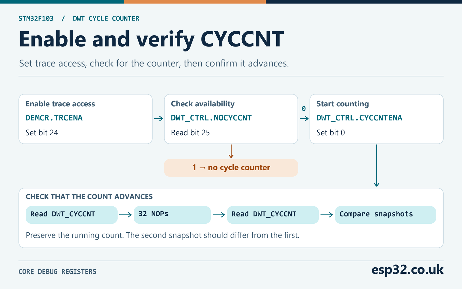
| CMSIS register or field | Role in the lab |
|---|---|
CoreDebug->DEMCR, bit 24 TRCENA | Enable access to the core trace blocks |
DWT->CTRL, bit 25 NOCYCCNT | Detect an implementation without CYCCNT |
DWT->CTRL, bit 0 CYCCNTENA | Start the cycle counter |
DWT->CYCCNT | Read the running 32-bit count |
Run this initialization from the normal privileged startup path. Core debug register access can be restricted by privilege, security state or implementation on other targets. STM32F103 also has separate STM32 debug configuration registers with their own behavior. For example, the applicable ST errata document describes a limitation on user software reading DBGMCU_IDCODE and DBGMCU_CR. The cycle counter routine uses the Cortex-M core registers named above and does not depend on reading either of those STM32 DBGMCU registers. ST STM32F103x8/B errata ES096
If the first attempt works only with a debugger attached, inspect the firmware’s initialization path. Some debug configurations touch trace settings on attach. Reset or power-cycle the board, let the firmware start, and read its saved result after the run. That checks whether the firmware itself set up the counter. A breakpoint inside the sampled interval stops normal execution. Use a breakpoint after the results are written and keep live memory polling, trace capture and single stepping out of the timing run as far as practical. ST debug toolbox application note AN4989
Place the measurement boundaries
The timing wrapper completes earlier explicit memory accesses with a data synchronization barrier, then uses an instruction synchronization barrier before reading the start count. It calls the chosen workload and executes a second data synchronization barrier before reading the end count. The preamble is before the start snapshot, so it is outside the measured window. The indirect call, return path and final barrier are within the bracket. The end barrier makes the measurement include completion of preceding explicit memory accesses from the core’s point of view, which matters for the GPIO comparison.
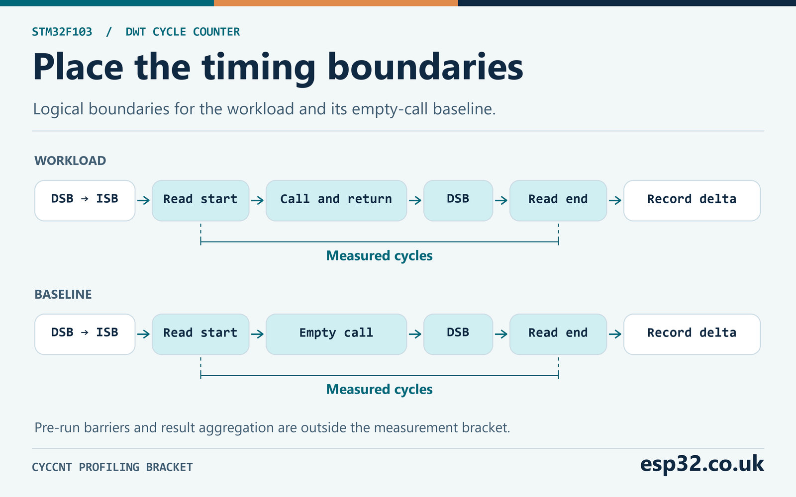
The CMSIS registers are volatile so the compiler emits the accesses. The empty GNU assembly statement with a memory clobber also constrains compiler motion of memory operations across the start boundary. That compiler barrier emits no processor instruction. The data synchronization barrier has an architectural effect. For a different benchmark containing pure arithmetic, make the input and result meaningful to the caller and verify the emitted instructions. A memory clobber by itself cannot guarantee that a constant expression will be recomputed between the snapshots.
The first workload is an empty function called through the same measurement wrapper. Its result includes snapshot and call machinery and the final barrier. Treat that reading as a measured reference for this build. Subtracting it gives an estimate of the additional work for another function. The final barrier may have to wait longer in the GPIO workload, and instruction placement or alignment can change between functions. Keep the raw result and the baseline alongside any adjusted number so a reader can see the size of that estimate.
The second workload uses GNU assembler’s repetition directive to emit exactly 32 NOP instructions. It gives the counter something deterministic to time while avoiding I/O. The source and linked disassembly can verify the number of instructions. The observed difference from the empty reference may also include fetch effects or an interrupt, so check that it is plausible and repeatable on your build. If the empty and NOP samples are identical across repeated runs, inspect the code and the two counter reads before interpreting any GPIO results.
| Workload | Operations in each sample | What it helps reveal |
|---|---|---|
| Empty call | Dispatch, return and measurement machinery | Baseline and measurement noise |
| 32 NOPs | Same call shape plus a fixed instruction block | Counter movement and a check against disassembly |
| HAL GPIO | 32 PB0 set/reset pairs through HAL | HAL call and branch overhead plus the GPIO writes |
| Direct BSRR | 32 PB0 set/reset pairs with register stores | GPIO stores and loop overhead in the direct path |
Make a fresh snapshot for each independent sample. The lab warms all four paths, then interleaves the four workloads in each of 64 trials. Running them in an interleaved order reduces the chance that a condition changing over the course of the run affects only one group. This also means the minimum for one workload may come from a different trial from the minimum for another. A difference between those minima is a comparison of the best observed cases, with each path measured independently.
In the linked build for this lab, the compiler inlined the measurement wrapper into Profile_Run. The disassembly shows the initial barriers, a load from DWT offset four, the indirect call, the closing DSB and a second load from DWT offset four before subtraction. It also scheduled a loop-index update between the final barrier and the end read. This is one reason to keep the raw baseline. The exact bracket contains the instructions emitted by that compiler, including bookkeeping it placed there. A source comment or a line boundary in the debugger will not tell you where each instruction ended up.
When reading a different disassembly, first locate the symbol for your timing routine. If it has been inlined, find the caller and look for the DWT base address 0xE0001000 and a load at offset four. Match that sequence to the indirect workload call or to the workload instructions themselves. Make sure there are two distinct reads and that the stores or computations you want to time are between them. Compare the ELF that is actually on the board with the file you are disassembling. An old image loaded through a previous debug configuration can give plausible numbers for the wrong implementation.
Convert cycles to time and handle rollover
At a fixed clock rate, divide cycles by HCLK to get seconds. Multiply by a million before dividing for microseconds, or by a billion for nanoseconds. HCLK is the Cortex core clock on this F103 setup. GPIOB is clocked on APB2 and timers can have their own clock rules. Those clocks affect how long parts of the workload take. The time conversion for DWT samples still uses the processor clock. The lab stores hclk_hz in the result so the number stays tied to the cycle count it describes.
| Cycles | HCLK | Calculation | Duration |
|---|---|---|---|
| 32 | 8 MHz | 32 ÷ 8,000,000 s | 4 µs |
| 32 | 72 MHz | 32 ÷ 72,000,000 s | About 444 ns |
| 144 | 72 MHz | 144 ÷ 72,000,000 s | 2 µs |
| 320 | 72 MHz | 320 ÷ 72,000,000 s | About 4.444 µs |
| 72,000 | 72 MHz | 72,000 ÷ 72,000,000 s | 1 ms |
The values in the table illustrate arithmetic. They are independent of any measured GPIO result. At 72 MHz one cycle is about 13.89 ns, so printing a whole number of nanoseconds gives readable units while the cycle count still sets the basic resolution. Oscillator accuracy and the exact placement of the snapshots also affect the interpretation. The conversion routine first promotes cycles to 64 bits, then multiplies, adds half the clock rate for nearest-integer rounding and divides. Keep division and string formatting outside the sample.
Rollover happens when the count goes from 0xFFFFFFFF to zero. Subtract the start from the end as unsigned 32-bit values. For example, starting at 0xFFFFFFF0 and ending at 0x00000020 gives 0x00000030, or 48 cycles. The modulo subtraction represents elapsed time correctly if the true interval is less than one complete counter period. A span of exactly one period returns zero, which is indistinguishable from equal snapshots taken without a wrap. Avoid trying to infer the number of missed wraps from two values alone.
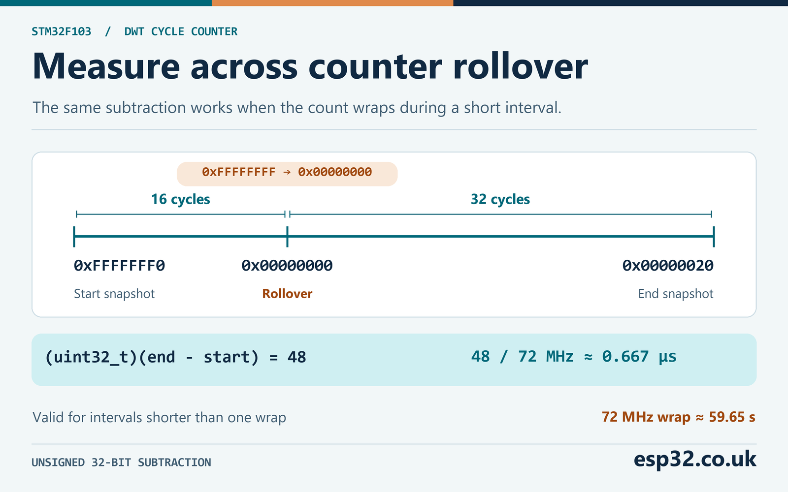
At 72 MHz the wrap period is about 59.65 seconds. At 8 MHz it is about 536.87 seconds. Those numbers are for a continuously running counter with a constant clock. If the CPU changes clocks during a measurement, a single HCLK value no longer describes the whole interval. Split the measurement into phases with known clocks or use a timebase appropriate to the application. For a timestamp spanning sleeps or extended debugger halts, choose and verify a clock that actually keeps running through the interval. STM32 low-power modes guide
For a data sheet or test log, retain the integer cycles and convert only when producing the report. Averaging rounded nanoseconds can introduce an avoidable rounding error. For instance, 32 cycles at 72 MHz round to 444 ns, whereas two batches totaling 64 cycles round to 889 ns. Accumulate the cycles first, then apply the conversion appropriate to the reported statistic. The helper accepts a 32-bit cycle delta. If you are converting a total from many intervals, use arithmetic sized for that total or divide into individual samples before applying the helper.
The counter is free-running throughout the benchmark. The result buffer contains separate short deltas, so the absolute value of CYCCNT at the beginning of a later trial is unimportant. To follow a long-running process in software, collect snapshots at known intervals shorter than one wrap and accumulate the deltas in a wider integer. A periodic sample must be guaranteed to arrive on time even when other work is busy. For long physical measurements where the clock can change or stop, count from an independent timebase with the required range.
Run the benchmark with STM32Cube HAL
Copy dwt_lab.h into the project’s include directory and dwt_lab.c into its sources. The module uses the CubeF1 HAL header for the GPIO driver and the device CMSIS header included by it. The example is written for a GCC-based STM32 project, which supports the inline assembly syntax in the NOP function. Use the generated startup and system code for your chip. Keep the default privileged foreground execution model and confirm PB0 is a low output before the call.
#ifndef DWT_LAB_H
#define DWT_LAB_H

#include <stdint.h>

typedef enum {
    PROFILE_OK, PROFILE_ARGUMENT, PROFILE_NO_COUNTER, PROFILE_STOPPED
} ProfileStatus;

typedef enum {
    PROFILE_EMPTY, PROFILE_NOP32, PROFILE_HAL_GPIO, PROFILE_BSRR, PROFILE_JOB_COUNT
} ProfileJob;

enum { PROFILE_TRIALS = 64, PROFILE_GPIO_PAIRS = 32 };

typedef struct {
    uint32_t min_cycles;
    uint32_t max_cycles;
    uint64_t total_cycles;
} ProfileStats;

typedef struct {
    uint32_t hclk_hz;
    uint32_t trials;
    ProfileStats job[PROFILE_JOB_COUNT];
} ProfileResult;

/* Call in privileged foreground code with PB0 configured as a low output. */
ProfileStatus Profile_Run(uint32_t hclk_hz, ProfileResult *result);

/* Returns zero when hclk_hz is zero. */
uint64_t Profile_Nanoseconds(uint32_t cycles, uint32_t hclk_hz);

#endif
#include "dwt_lab.h"
#include "stm32f1xx_hal.h"
typedef void (*Workload)(void);
static void empty(void)
{
__asm volatile ("" ::: "memory");
}
static void nop32(void)
{
__asm volatile (".rept 32\n nop\n .endr" ::: "memory");
}
static void gpio_hal(void)
{
for (unsigned i = 0; i < PROFILE_GPIO_PAIRS; ++i) {
HAL_GPIO_WritePin(GPIOB, GPIO_PIN_0, GPIO_PIN_SET);
HAL_GPIO_WritePin(GPIOB, GPIO_PIN_0, GPIO_PIN_RESET);
}
}
static void gpio_bsrr(void)
{
for (unsigned i = 0; i < PROFILE_GPIO_PAIRS; ++i) {
GPIOB->BSRR = GPIO_PIN_0;
GPIOB->BSRR = (uint32_t)GPIO_PIN_0 << 16;
}
}
static ProfileStatus enable_counter(void)
{
CoreDebug->DEMCR |= CoreDebug_DEMCR_TRCENA_Msk;
__DSB();
__ISB();
if (DWT->CTRL & DWT_CTRL_NOCYCCNT_Msk) {
return PROFILE_NO_COUNTER;
}
DWT->CTRL |= DWT_CTRL_CYCCNTENA_Msk;
__DSB();
__ISB();
uint32_t before = DWT->CYCCNT;
nop32();
return DWT->CYCCNT != before ? PROFILE_OK : PROFILE_STOPPED;
}
static uint32_t measure(Workload run)
{
__DSB();
__ISB();
uint32_t start = DWT->CYCCNT;
__asm volatile ("" ::: "memory");
run();
__DSB();
return (uint32_t)(DWT->CYCCNT - start);
}
static void record(ProfileStats *stats, uint32_t elapsed)
{
if (elapsed < stats->min_cycles) {
stats->min_cycles = elapsed;
}
if (elapsed > stats->max_cycles) {
stats->max_cycles = elapsed;
}
stats->total_cycles += elapsed;
}
ProfileStatus Profile_Run(uint32_t hclk_hz, ProfileResult *result)
{
static const Workload workloads[PROFILE_JOB_COUNT] = {empty, nop32, gpio_hal, gpio_bsrr};
if (!result || !hclk_hz) {
return PROFILE_ARGUMENT;
}
ProfileStatus status = enable_counter();
if (status != PROFILE_OK) {
return status;
}
ProfileResult run = {.hclk_hz = hclk_hz, .trials = PROFILE_TRIALS};
for (unsigned job = 0; job < PROFILE_JOB_COUNT; ++job) {
workloads[job]();
run.job[job].min_cycles = UINT32_MAX;
}
for (unsigned trial = 0; trial < PROFILE_TRIALS; ++trial) {
for (unsigned job = 0; job < PROFILE_JOB_COUNT; ++job) {
record(&run.job[job], measure(workloads[job]));
}
}
*result = run;
return PROFILE_OK;
}
uint64_t Profile_Nanoseconds(uint32_t cycles, uint32_t hclk_hz)
{
if (!hclk_hz) {
return 0;
}
return ((uint64_t)cycles * UINT64_C(1000000000) + hclk_hz / 2U) / hclk_hz;
}Declare the watch variables in a generated file’s user section, then place the executable portion after the generated GPIO and clock initialization. Include the normal CubeMX call to SystemClock_Config() if the project generates it. SystemCoreClockUpdate() refreshes the CMSIS value from the configured clock tree. Its output depends on the configured oscillator constants, so confirm that any external crystal and project settings agree. The two code files leave pin setup with the application, which makes it easy to check who owns the output in a larger project.
#include "dwt_lab.h"

volatile ProfileStatus profile_status = PROFILE_STOPPED;
volatile ProfileResult profile_result;
volatile uint32_t profile_done;

/* After HAL, system clock and GPIO initialisation */
SystemCoreClockUpdate();
ProfileResult run;
profile_status = Profile_Run(SystemCoreClock, &run);
if (profile_status == PROFILE_OK) {
    profile_result = run;
}
profile_done = 1;
/* Continue into the generated main loop. */
Flash and run at full speed until profile_done is one. Halt outside the timed code and inspect profile_status first. With a successful run you should see the HCLK value, the trial count and four statistics entries. For each workload, min_cycles and max_cycles report the extrema, while total_cycles contains all 64 samples added together. Divide the total by the number of trials to compute the mean. The struct contains raw cycle values. You can call the nanoseconds conversion on a selected sample after the measurement or perform the arithmetic later in a worksheet.
The result is copied into the debugger-visible variable only after the run succeeds. If the caller supplied a zero frequency or the counter failed to start, profile_done still indicates completion and profile_status indicates the failure. If you adapt the one-shot code to run periodically, arrange that readers see a complete record. For example, a logging task can take a copy after the profiling task finishes and posts a message. The volatile watch variable in this example is for inspection after the run. It does not make a multiword structure update atomic.
Here is an example of how to read one statistics row. If a workload recorded a total of 23,040 cycles in 64 trials, its mean would be 360 cycles. If the minimum were 340 and maximum 610, a short table should show all three values. Averages alone hide the difference between a consistently slower path and an otherwise fast path that occasionally gets interrupted. The pair count and HCLK belong beside the statistics. With a 72 MHz clock, 360 cycles corresponds to 5 µs for the whole measured sample, before any baseline adjustment.
To find what produced a long sample, temporarily extend the test to save the individual deltas in a buffer after each end snapshot. The buffer lets you look at the distribution or correlate the sample order with activity elsewhere in the application. Keep the trace storage outside the timing bracket. Extra writes between samples can still shift when the next sample begins relative to SysTick. Treat the capture build as another measurement configuration and save enough information to reproduce it.
Compare HAL and BSRR on the same pin
On STM32F103, writing a one in the lower half of GPIOB_BSRR sets the corresponding output latch bit. Writing a one in the upper half resets that bit. The lab sets PB0 with 0x00000001 and resets it with 0x00010000. The HAL GPIO driver also writes BSRR for the set and reset operations in this version. Each workload makes the same 32 pairs of writes and ends with PB0 low. A write-only BSRR operation avoids a read-modify-write on the whole output register and leaves other port bits alone. ST STM32F1 GPIO HAL v1.1.10
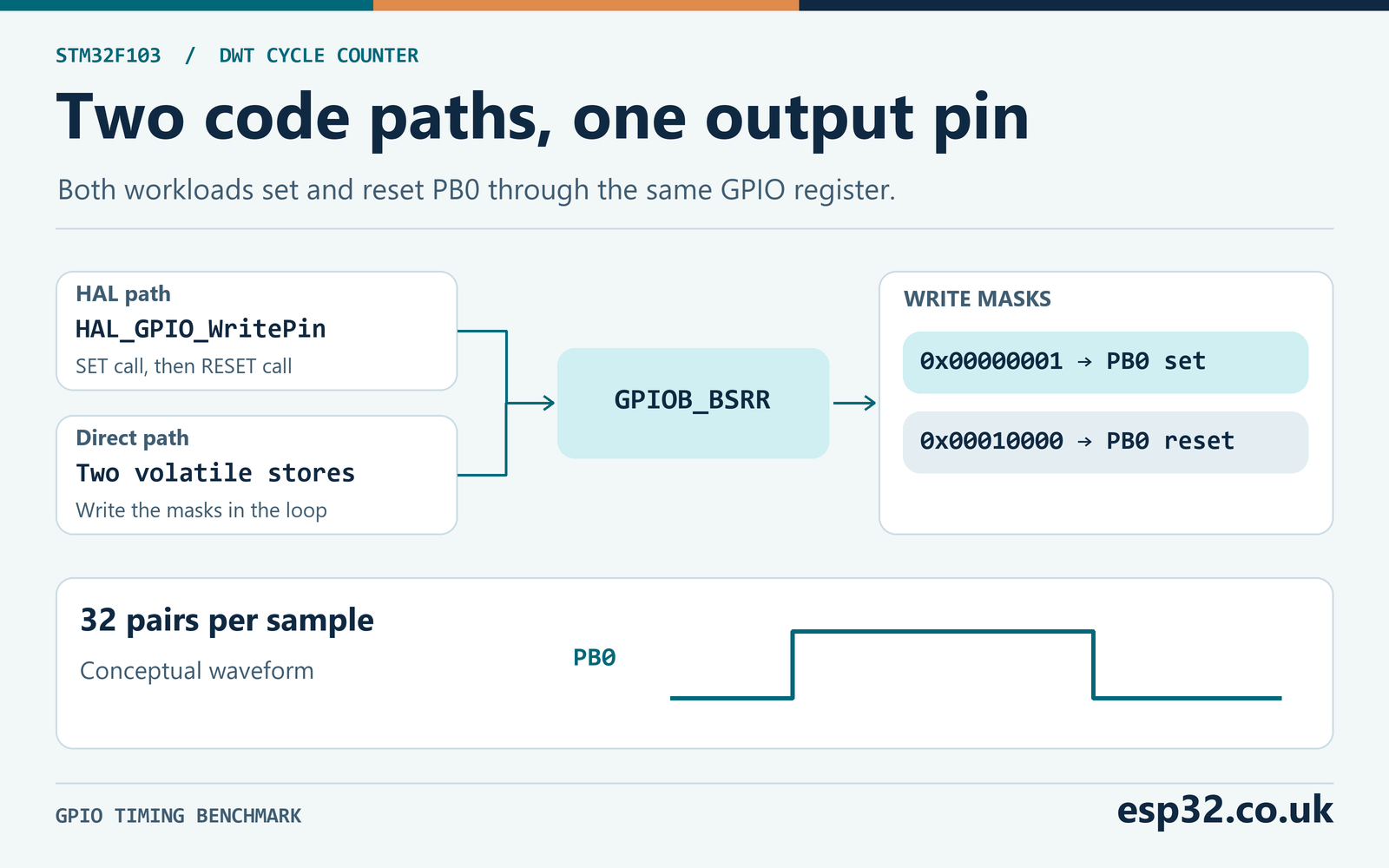
The HAL path passes a port pointer, a pin mask and a pin state into a function twice per pair. The direct path writes the two masks to the register inside its own loop. Look at the linked disassembly to see whether each HAL call survived optimization. For example, a build with link-time optimization could inline the HAL implementation and remove much of the difference between the paths. The comparison is meaningful for a stated build, optimization setting and workload. The code uses the same GPIO and clock configuration in both cases, so changing those settings between paths would weaken the comparison.
Report the pair count with the result. If an illustrative empty minimum were 20 cycles and a 32-pair workload minimum were 340 cycles, the additional work would be about (340 − 20) ÷ 32 = 10 cycles per pair. At 72 MHz that is about 139 ns per pair. This example explains the arithmetic only. The pair result still includes loop control, bus waits and the contribution of the final barrier averaged across the batch. Dividing a pair by two gives an arithmetic average per operation. It does not determine the separate latency of the set and reset paths.
The oscilloscope shows successive rising and falling edges. High pulse width measures the interval from a rising threshold crossing to a falling threshold crossing. A period between two rising edges spans a complete pair of writes and the loop path between them. The DWT bracket also includes the measurement call, return and barrier, and the first and last edges in a finite burst do not bound exactly the same work. Compare repeated pulse periods to the approximate per-pair calculation. Use the scope to report electrical details such as edge rate, ringing and actual minimum pulse width.
To isolate a different cost, change the workload deliberately. A single set/reset pair makes function call and measurement overhead proportionally larger. A longer batch improves the granularity of cycles per pair, but it also raises the chance that an interrupt lands inside the sample. If the workload needs a particular bus or GPIO state to be representative, initialize that state before the start snapshot and describe it with the measurement. For a heavily loaded application, run a second batch with normal peripherals active and compare its spread with the bare bench run.
The linked GPIO routines show useful differences you can check before ever connecting the scope. The direct loop loads the GPIOB base and stores both mask values at the BSRR offset of 16 bytes. The HAL loop branches to HAL_GPIO_WritePin twice and passes the requested state each time. The linked HAL function selects the mask operation and performs the store. These instructions establish what the firmware attempts to do. A physical capture is the check that PB0 has the expected electrical behavior with the chosen speed, voltage, probe and load.
Count the edges if the captured bursts are hard to distinguish. Each GPIO workload produces 32 intended rising and 32 intended falling transitions. The warm-up also drives the pin before the 64 interleaved trials begin. A wide capture can therefore contain several bursts and gaps while the empty and NOP workloads run. If you need an unmistakable single burst for debugging, temporarily run just one GPIO path once, then restore the full benchmark for the statistical comparison. Label any screenshot with the version that produced it.
Interpret variation before claiming a speedup
SysTick and any enabled interrupts can preempt a timed foreground function. CYCCNT can then include exception entry, handler work and return within the bracket. A higher maximum with a stable minimum is a reason to inspect interrupts and bus activity. It can also reflect genuine path variation. Sixty-four samples are a useful quick look, with no guarantee of capturing every rare event. If worst-case execution time matters, instrument the production workload, include competing activities and make the timing argument from the full system design.
For an isolated experiment, you can repeat the lab with maskable interrupts temporarily disabled. Save the existing PRIMASK and restore it after the shortest practical measurement window. Keep delay functions and operations that depend on interrupts outside that window. System faults and NMI are separate from normal maskable interrupts. Record whether masking was used and treat the result as a separate condition. The supplied firmware leaves the HAL tick and normal interrupt handling intact so its measurements also show scheduling noise that occurs naturally.
Compare release and debug builds by recording the optimization option and LTO state. A debugger attached to an optimized build can make source stepping misleading because instructions are reordered and variables may live in registers or disappear. Disassemble the exact ELF that was flashed and check the code between the reads. If comparing algorithms, feed equivalent inputs, verify equivalent output and keep setup, allocation and result printing outside the bracket unless those are part of the task under measurement.
| Symptom | Check first |
|---|---|
PROFILE_NO_COUNTER | Confirm the actual processor and its documented DWT implementation |
PROFILE_STOPPED | Check the startup path, privilege, trace enable and whether the core ran freely |
PROFILE_ARGUMENT | Supply a result buffer and the actual nonzero HCLK |
| Valid counts with implausible times | Check the HCLK value, unit conversion and oscillator constants |
| Rare long samples | Look for interrupts, debugger activity, stalls and other bus traffic |
| HAL and BSRR very close | Inspect inlining, LTO, loop shape and the amount of common overhead |
| Missing pulses on the scope | Check GPIOB clock, pin mode, probe point and single-shot trigger timing |
| Small or zero delta for a long interval | Check elapsed duration against the counter wrap period |
Record enough detail to reproduce the result after changing the firmware. Keep the board and MCU marking, clock source, HCLK, APB2 prescaler, Flash latency, build flags, workload count and interrupt conditions with the four raw statistics. The supplied arithmetic works from those raw cycle counts. When you replace the GPIO workload with a parser, filter or ISR, carry the same discipline forward. Keep the input data and test boundaries visible, and use the electrical measurement when an external signal is the real timing requirement.