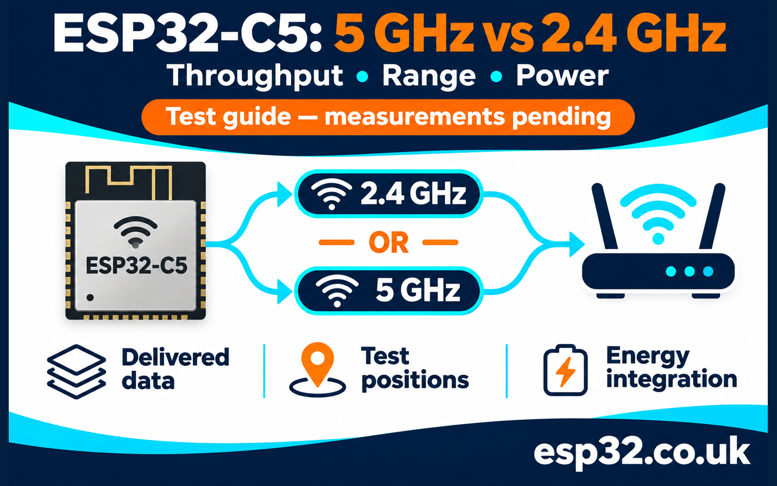
The ESP32-C5PriceAliExpress price gives an embedded project a useful choice: connect over 2.4 GHz or move onto 5 GHz. That sounds like a straightforward upgrade until you try to answer the questions that actually matter. Will a firmware upload finish sooner? Will a sensor remain connected through two walls? Will a battery last longer if a transfer completes quickly, even when the radio draws more current while transmitting?
There is no measured winner in this article yet. This is a practical test guide, with verified hardware capabilities, repeatable procedures and blank results tables. No throughput, distance or battery-life figures below represent tests performed by esp32.co.uk/. The aim is to make the eventual comparison useful enough to reproduce, rather than turn a chip specification into a performance claim.
You can follow the procedure with one C5 board, a dual-band router and a computer connected by Ethernet. A current logger adds the power comparison. Start with the networking tests if you do not have one; leaving an energy result empty is more informative than deriving it from an unrelated datasheet number.
What the ESP32-C5 actually supports
Espressif specifies a single transmit and receive chain supporting both bands. Its 802.11ax modes use 20 MHz channels; 802.11ac is also limited to 20 MHz, while legacy 802.11n supports 20/40 MHz operation. Dual-band support does not mean two independent Wi-Fi links running simultaneously. These distinctions come from the ESP32-C5 datasheet.
A router described as AX3000 or advertising 160 MHz channels cannot make this board use those capabilities. Its marketing total combines resources that your particular client cannot necessarily access. Record the C5 connection and the access point configuration separately. A router setting describes what the router permits; it does not prove which mode a transfer used.
Likewise, a physical-layer rate is not the rate at which your application receives useful bytes. Protocol headers, acknowledgements, contention, retransmission and software processing all consume time. The comparison here measures delivered traffic across a local network, then checks whether that result survives the conditions of a real installation.
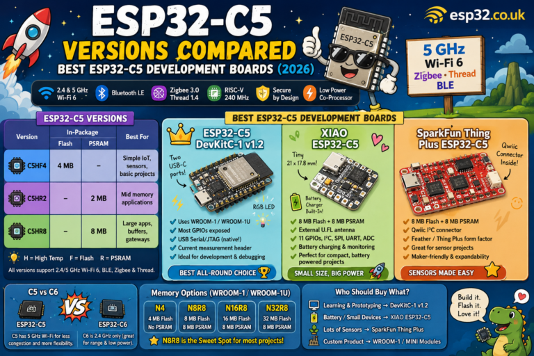
If you are still choosing hardware, the existing ESP32-C5 board guide covers the purchasing context. For this experiment, use the same physical board for both bands. Comparing two different boards would introduce antenna, regulator and layout differences before the Wi-Fi test had even started.
Define the question before selecting the settings
There are two worthwhile comparisons. The first asks how the bands behave under a matched configuration: the same board, location, traffic direction, 20 MHz channel width and power policy. This helps explain whether changing band improves a particular connection. The second asks which configuration works best for the finished project, including its actual firmware, enclosure and router settings.
Run those as separate experiments. If you optimise the 5 GHz configuration but leave 2.4 GHz at an unsuitable default, the result describes your settings as much as the bands. That may still be useful for a deployment decision, but it needs a clear label. Even with matched settings, different router radios and antennas remain part of the test system.
Write a short acceptance statement before collecting results. For an update service, it might be that a fixed payload must finish within a chosen time with no disconnects. For a sensor, it might be that every scheduled message receives an application acknowledgement before its deadline. Specify your own payload and deadline rather than adopting arbitrary limits from a throughput chart.
Choose the decision rule now as well. A high median with repeated failures may be worse than a slower connection that completes every run. Keeping reliability beside speed prevents an attractive best-case result from hiding the behaviour that will cause maintenance calls later.
Build a local test network
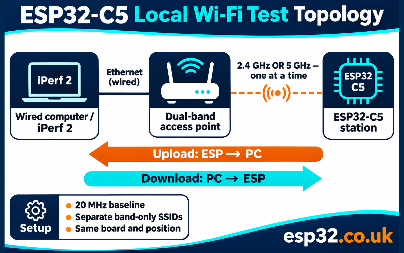
Connect the computer running the test server to a LAN port on the router by Ethernet. Disable that computer’s Wi-Fi for the experiment and verify which network interface holds its server address. The C5 should be the only wireless hop in the measured path. A wireless laptop server would make two radio links compete and leave you unsure which one limited the result.
Keep the traffic inside the LAN. An internet speed test adds the broadband connection, a remote server and routing outside your control. It can be useful for checking internet access, but it cannot isolate the C5 link. A local test also allows you to repeat measurements when the internet connection is unavailable.
Use one access point in a fixed position. Avoid mesh roaming during the baseline test, and keep the server out of a guest network with client isolation. Allow the selected iPerf service through the host firewall only on the trusted test network. Do not expose a benchmark server to the internet or disable the firewall globally.
Mark the board position on a nonconductive stand. Keep its height, antenna orientation and USB lead routing consistent. Move your hands away before each run. Record the router model, firmware, Ethernet link speed and approximate room conditions. These details help explain a later change without pretending that a domestic room is a calibrated RF chamber.
Make the two bands unambiguous
Create separate test SSIDs, such as C5_TEST_24 and C5_TEST_5, each broadcast on its intended band only. Disable automatic band steering for this test. Reusing one SSID across both bands is convenient in normal operation, but it makes a controlled comparison harder because association policy can choose a different radio without an obvious change to the network name.
Configure a 20 MHz baseline on both radios where the router permits it. Keep security settings comparable, and use a fixed channel for each band if the access point supports that. Leave the router configured for its actual country and use channels permitted by the equipment and local rules. Record the actual operating channel after association, including any automatic change.
Do not treat channel number, SSID or RSSI alone as a complete connection record. Save the access point’s BSSID as well, so a mesh node or second router cannot silently enter the comparison. Router client information can supplement the firmware log, but distinguish reported capabilities from an observed negotiated mode.
Test both SSIDs at the starting position before walking away. If one does not appear, resolve discovery, channel, security and firmware issues there first. A connection that cannot be established beside the router has not provided evidence about the range of that band. Log it as a setup problem until you know otherwise.
Freeze the firmware and tools
This procedure uses Espressif’s ESP-IDF v5.5.1 iPerf example as a named baseline, rather than assuming that every SDK release behaves identically. The versioned README lists ESP32-C5AliExpress price support and specifies iPerf 2.x compatibility. Install iPerf 2 on the computer; an executable named iperf3 is a different protocol implementation.
Open the ESP-IDF terminal for that release. Copy the example into a new working folder so your experiment has its own configuration. The following shell commands assume an activated ESP-IDF environment with Python and Git available. In PowerShell, use its normal folder-copy command in place of cp.
idf.py --version
git -C "$IDF_PATH" describe --tags --always --dirty
cp -R "$IDF_PATH/examples/wifi/iperf" ./c5-band-test
cd c5-band-test
idf.py set-target esp32c5
idf.py menuconfig
idf.py build
idf.py -p YOUR_SERIAL_PORT flash monitor
Replace YOUR_SERIAL_PORT with the port belonging to your board. Select the console interface you actually connected in menuconfig; a UART bridge and native USB Serial/JTAG are different paths. Save the console help output, resolved dependency lock file, final sdkconfig, build log and firmware binary with the session. Also retain the example’s main/idf_component.yml: its versioned dependency manifest allows compatible component updates. The SDK tag alone does not freeze managed component versions.
Espressif’s example defaults include benchmark-specific settings, disabled watchdog settings and experimental PHY options. Preserve and disclose the effective configuration for a baseline, then restore production safeguards when building the real application. A benchmark example is a laboratory workload. It has not been built or flashed for this article, and its settings should not become an unreviewed production template.
Record power policy and association state
Use a clearly named firmware profile for each experiment. For the throughput baseline, explicitly disabling Wi-Fi modem sleep removes one variable. For the application energy test, use the power policy your application intends to ship. Apply the same policy to both bands within a comparison, and record CPU settings, logging level and other active radios.
In a project you control, these are the relevant operations after Wi-Fi driver initialisation. They are integration snippets, not a replacement for the example’s startup and event handling. Run the policy call before the timed test, and query association information only after the station has connected. Check errors rather than continuing with an assumed configuration.
#include "esp_err.h"
#include "esp_wifi.h"

/* After Wi-Fi initialisation, before the timed baseline. */
ESP_ERROR_CHECK(esp_wifi_set_ps(WIFI_PS_NONE));

/* In task context after association; save these fields in the run log. */
wifi_ps_type_t actual_ps;
wifi_ap_record_t ap = {0};
ESP_ERROR_CHECK(esp_wifi_get_ps(&actual_ps));
ESP_ERROR_CHECK(esp_wifi_sta_get_ap_info(&ap));
/* Record actual_ps, ap.bssid, ap.primary and ap.rssi. */
The versioned Wi-Fi header defines these APIs. Espressif’s power-save guide explains the modem-sleep trade-off: waking according to access point timing can save energy while adding receive delay. That guide is v6.0; the executable baseline here remains v5.5.1. Keep version differences visible when adapting the procedure.
Place those statements inside your existing initialisation and connected-task functions, respectively; they are not valid as standalone file-scope statements. Capture association data before and after a run rather than printing continuously in the traffic path. Do not perform repeated network scans during a timed transfer. If the firmware cannot report a negotiated detail reliably, mark that field unavailable and retain the evidence it can provide. Guessing a mode from the router’s product name weakens the record.
Establish a clean first connection
At the ESP console, inspect help before entering test commands. Join the 2.4 GHz test network first, substituting a temporary test password. Keep credentials out of anything you later publish; serial transcripts and configuration files can contain them.
help
sta_connect C5_TEST_24 YOUR_TEST_PASSWORD
Wait for association and an IP address. Record the ESP address, server address, BSSID, channel, power profile and firmware identifier. Confirm the server is reachable on the LAN. A failed ping can reflect firewall policy, so use it as a diagnostic clue rather than a universal requirement for iPerf to work.
Make one short untimed trial and check both ends of the transfer. Confirm that the computer is actually receiving data and that the displayed units make sense. Then leave the connection idle for a fixed settling interval, such as ten seconds. This is a procedural choice to keep runs comparable, not a guarantee that all rate adaptation has settled.
For the second band, stop active traffic, disconnect or restart the station using the commands exposed by that build’s help, and connect to C5_TEST_5. Verify the association again. A clean restart between band changes is acceptable if you use it consistently and exclude startup from the timed throughput measurement.
Measure TCP upload and download separately
Here, upload means ESP32-C5AliExpress price to the wired computer. Start the computer as an iPerf 2 server, then start the ESP client using the computer’s LAN address. The address below is an example and must be replaced with yours.
# Wired computer
iperf -s -i 3
iperf -c 192.168.10.42 -i 3 -t 60Use a 60-second timed run and retain the complete log. Record the receiver’s final bytes and interval where available. For manually calculated goodput, divide delivered bytes by the corresponding measured duration, multiply by eight and divide by one million for decimal Mbit/s. Keep sender and receiver reports labelled; their intervals can differ slightly.
Download reverses the roles. Stop the PC server before starting the PC client, and stop the previous ESP session before starting its server. The component’s documented console syntax includes server mode and an abort command; confirm the resolved component exposes them in help.
iperf -s -i 3# Wired computer; replace with the ESP address
iperf -c 192.168.10.77 -i 3 -t 60Do not substitute an iPerf 3 reverse-mode command. Explicit client and server roles make the direction clear and avoid depending on an unsupported option. Keep one stream for the baseline. If you later investigate multiple streams, label that as another experiment instead of merging its results with the single-stream set.
Complete five runs per band and direction at each chosen position. Alternate band order between paired repeats, and use the same rest interval. Report the median, minimum and maximum across valid completed runs, together with completed attempts over total attempts. A failed run remains a failure record; do not replace it with a fresh run and quietly discard the original.
Use UDP to investigate offered load and loss
TCP is useful for bulk transfers because it responds to delivery conditions. UDP answers a different question: what happens when the sender offers a specified rate without TCP’s congestion control? A high send rate is not evidence that the receiver obtained that traffic. Always retain the receiver’s report, particularly when the sender appears to sustain an impressive rate.
Start with a low offered load, then increase it in a predeclared sequence. For example, try 1, 2, 5 and 10 Mbit/s before deciding whether further steps are useful. Those are test inputs, not predicted C5 results. Keep datagram length fixed and below the path MTU; 1200 payload bytes is a practical starting choice for this IPv4 LAN test.
For an ESP-to-PC trial, run a UDP server on the wired computer. In the documented ESP component interface, bandwidth is expressed in Mbit/s as a number; the following ESP command requests one Mbit/s. Check help on your resolved version before using it.
# Wired computer
iperf -s -u -i 3
iperf -c 192.168.10.42 -u -b 1 -l 1200 -i 3 -t 60Record offered load, received goodput, received and missing datagrams, loss percentage and receiver-reported jitter if available. Jitter here is a tool-specific network statistic, not a guaranteed bound on application response time. If the ESP receiver does not expose the metrics you need for a reverse UDP experiment, leave them unavailable rather than reconstructing loss from the sender’s byte counter.
A reverse UDP test can be useful, but validate its reporting before adding it to the comparison. Keep its command syntax and units separate from the ESP console: desktop iPerf 2 commonly accepts values such as 1M. Never assume that a bandwidth argument copied between two implementations has identical units.
Turn range into a repeatable service test
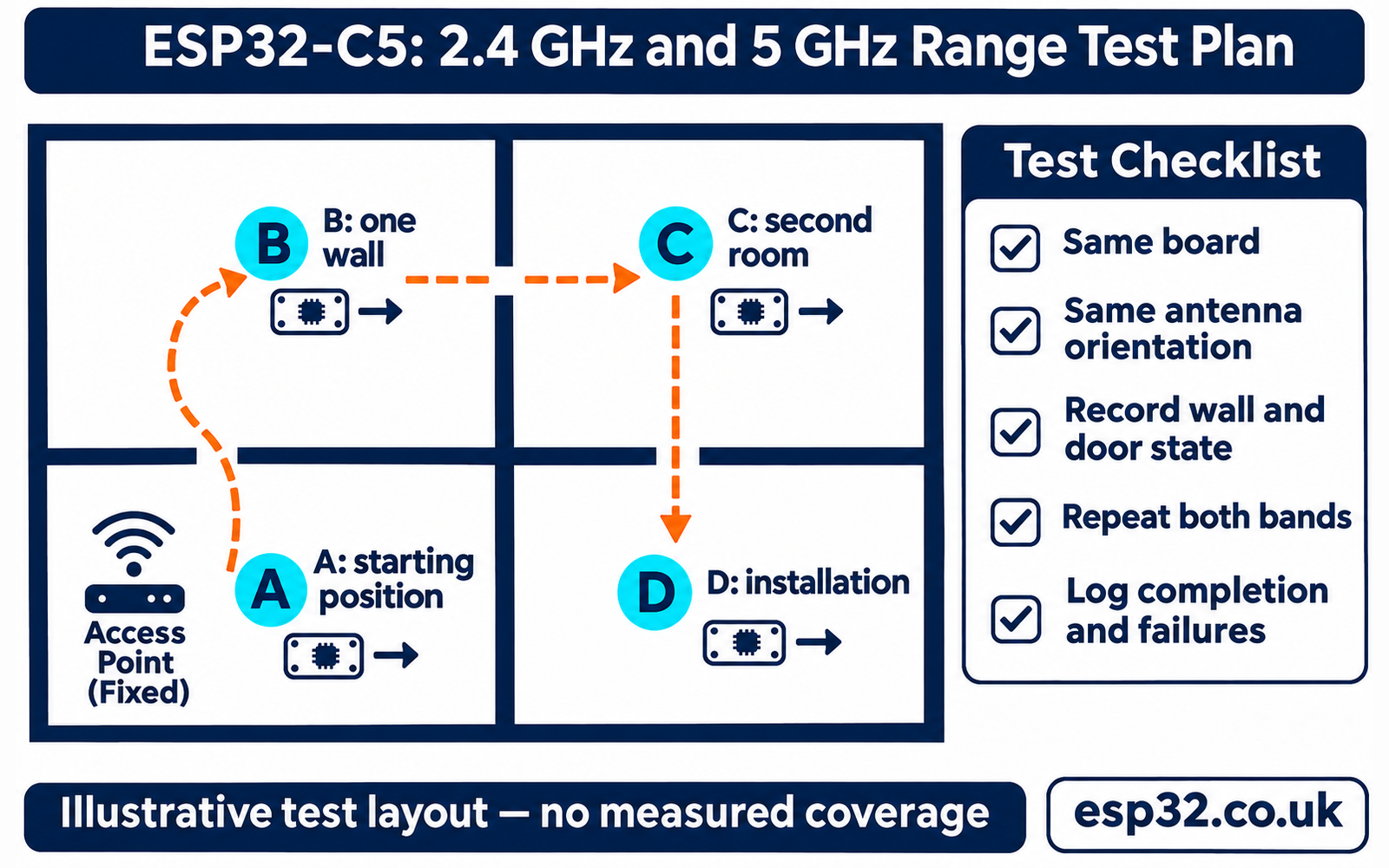
A maximum distance without a workload definition is difficult to use. A board may remain associated while transfers repeatedly stall. Define useful range as the set of marked locations where your application meets its delivery and timing requirements. Keep a separate record of association success so readers can see the difference between finding an access point and completing useful work.
Choose a small set of realistic positions: an unobstructed starting point, one intervening wall, a second room and the intended installation position. Measure distances if practical, but also record wall type, approximate board height, orientation and door state. These descriptions make a domestic test more informative without suggesting precision the environment cannot support.
Move the same board along the same route for both bands. At each position, repeat the connection check and the chosen workload. Fix a connection timeout in advance. A timeout should create a recorded failed attempt, not an indefinite wait until a connection eventually appears. If the route changes, start a new session rather than appending incompatible readings.
In ideal free space, doubling frequency adds about six decibels of path loss with equal distance and antenna gains. Real rooms add reflections, absorption, interference and unequal antenna patterns. That simple calculation explains why a band change can alter the link budget; it cannot predict how many walls your board will cross or identify a universal distance limit.
Read RSSI alongside delivery evidence
RSSI helps describe what changed, but it is not a throughput measurement. A strong received signal can coexist with heavy channel contention. A weaker signal may still carry a small sensor payload reliably. Record RSSI using the same device and method, and avoid comparing its absolute value directly with a phone or a different board.
Take a reading before and after each run. If you have a sampling logger, retain its sampling interval and avoid allowing the logger to become the main workload. Pair those readings with completion status, receiver goodput and disconnect events. A sudden change in channel or BSSID deserves investigation before the run is compared with its neighbours.
Do not smooth failures out of a range chart. A useful presentation shows completed attempts and failed attempts at each position, then summarises speed only for the completed set. That leaves the trade-off visible: one configuration might transfer quickly when it works but fail too often for an unattended installation.
Measure power at a stated boundary
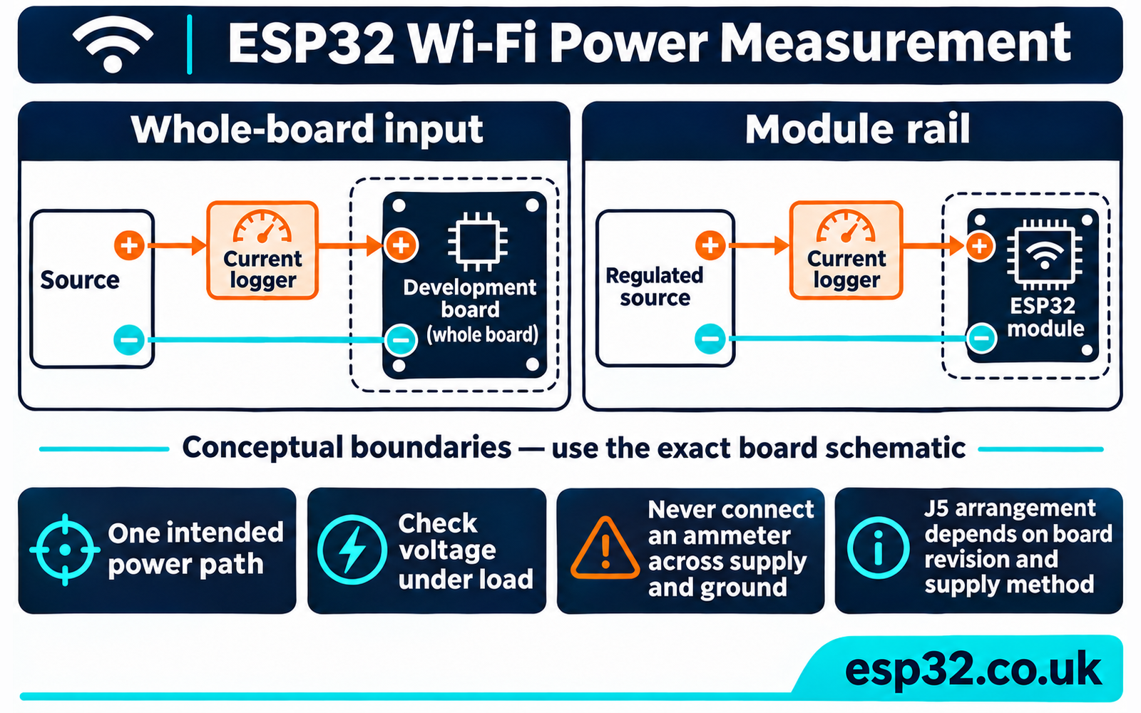
First decide whether you are measuring a development board or its module. A USB-side measurement includes conversion losses and other powered board circuitry. A module-rail measurement answers a narrower question. Both can be useful, but they should have different labels and should never be combined into one average.
On Espressif’s C5 DevKitC-1 v1.2, the official board guide identifies J5 for module-current measurement. With power off, remove the jumper and insert a suitably rated measuring instrument in series across that measurement path. Follow the guide for your exact board revision; feeding the 3V3 header bypasses J5 and requires a different arrangement.
Never place an ammeter directly across a supply and ground. Check its range, burden voltage and transient capability before energising the board. Use one intended power source, avoid backfeeding through another USB connection and keep the wiring short. If a USB data connection remains attached, establish whether it introduces an additional power path before trusting the reading.
Record supply voltage at the board during activity, not just the unloaded supply setting. A measurement device that drops too much voltage can create resets or retries and change the network behaviour it is meant to observe. Compare an instrumented networking trial with the original baseline before accepting the power setup.
Compare energy for the same completed job
Collect three different workloads: associated idle, sustained traffic and a fixed application job. State whether idle still includes periodic logging or background traffic. For sustained traffic, align the power capture with the network measurement window. Report instrument sampling rate and integration method; a slow display cannot characterise short current peaks.
For a fixed job, choose a payload large enough to measure reliably and verify that the receiver actually accepted it. A local HTTP transfer with a length and checksum check is one possible application test, but it is separate from the stock iPerf workload and requires its own implementation. Do not call an iPerf byte stream a verified firmware-update transaction.
Integrate power over the whole declared window: energy in joules is the integral of voltage multiplied by current over time. If voltage is sufficiently constant, a logged average current multiplied by measured voltage and duration is an approximation; disclose that assumption. Convert milliamps to amps before multiplying. Joules per delivered megabyte requires a stated decimal or binary byte convention.
For battery-oriented devices, include wake-up, association, transfer, acknowledgement and the return to sleep in the job window. For a continuously connected device, use a fixed observation period with the same task schedule. State which boundary you used so a quick transfer is not rewarded by excluding its connection overhead.
A band could draw more power during a successful transfer and still consume less energy for that completed job. It could also lose that advantage when connection attempts or retransmissions increase. These are hypotheses for the measurement to resolve. Do not estimate a winner by multiplying a datasheet RF current by a guessed transfer time.
Repeat the test with the application workload
After the isolated networking baseline, restore the tasks that will run in the finished device. Keep the same locations and repeat the acceptance test with sensors, display updates, encryption and background processing active as appropriate. Save this as an application profile with its own firmware identifier. Do not merge it with the benchmark profile, even when both use the same SDK.
For periodic telemetry, choose a fixed payload, sending interval and acknowledgement deadline. Count every scheduled job, including messages that never reach the application server. Record how many finish on time, how many finish late and how many fail. A transport connection remaining open does not prove that a downstream automation received or acted on the message.
For an update download, time a fixed, verified file and retain the server-side byte count and device-side verification outcome. Use the security configuration intended for deployment. A plaintext throughput test can describe a radio path, but it cannot establish completion time for an encrypted update that also performs flash writes and signature checks.
Choose a fixed observation duration before the run and keep it identical across bands. For a sleeping device, include complete repeated wake-and-send cycles rather than selecting only the cleanest transfer. For an always-connected device, include the normal gaps between messages. This reveals whether idle time, reconnects or the transfer itself dominates the energy budget. If either firmware profile behaves differently when the measurement instrument is attached, resolve that discrepancy before comparing its energy result.
Keep blanks, failures and measurements distinct
The following tables are deliberately unfilled. An empty measurement means no reading has been supplied. After testing, use a clear status such as completed, connection_failed or transfer_failed, and retain the raw log filename. Never insert zero to make a spreadsheet chart look complete; a zero measurement and an unperformed test have different meanings.
For TCP, enter the median and spread only after collecting the repeated runs. Completed attempts should remain visible alongside the summary. Keep upload and download rows separate even when their values happen to be similar.
| Position | Band | Direction | Completed / attempted | Median Mbit/s | Min–max Mbit/s |
|---|---|---|---|---|---|
| Starting position | 2.4 GHz | ESP to PC | |||
| Starting position | 5 GHz | ESP to PC | |||
| Starting position | 2.4 GHz | PC to ESP | |||
| Starting position | 5 GHz | PC to ESP | |||
| Installation position | 2.4 GHz | ESP to PC | |||
| Installation position | 5 GHz | ESP to PC |
For the UDP comparison, add a row for every offered load and position. Loss and jitter should come from a receiver that actually reports them. Label the direction and datagram length in the associated session record.
| Position | Band | Offered Mbit/s | Received Mbit/s | Loss % | Receiver jitter ms |
|---|---|---|---|---|---|
| Starting position | 2.4 GHz | ||||
| Starting position | 5 GHz | ||||
| Installation position | 2.4 GHz | ||||
| Installation position | 5 GHz |
For power, keep each measurement boundary and workload in its own row. A whole-board USB result belongs beside another whole-board USB result. Record a failed job’s energy too, with its failure status, so a retry-heavy configuration does not appear efficient through selective reporting.
| Boundary and workload | Band | Mean power mW | Duration s | Energy J | Delivered bytes |
|---|---|---|---|---|---|
| USB board, fixed job | 2.4 GHz | ||||
| USB board, fixed job | 5 GHz | ||||
| Module rail, associated idle | 2.4 GHz | ||||
| Module rail, associated idle | 5 GHz |
The accompanying CSV templates retain individual attempts and instrument details. Keep a fresh copy for each session, and archive the unedited logs alongside it. Summaries should be traceable to those records rather than to screenshots containing only a final headline number.
Troubleshoot the test before blaming the band
If 5 GHz is missing, check that the board is genuinely an ESP32-C5, the access point broadcasts the intended SSID, and the selected channel and security configuration are supported by the actual firmware. Confirm discovery at the starting position. Router channel changes or channel-availability delays can look like intermittent client faults; retain the access point log where available.
If neither direction transfers, check the server address, host firewall, guest isolation and iPerf version. If only one direction fails, inspect the client/server roles and whether an old server still owns the port. Stop previous sessions cleanly before restarting them. A routing or firewall failure should not become a zero-throughput result attributed to RF performance.
If speed is unexpectedly low, inspect the wired server first. Check Ethernet negotiation, CPU load and simultaneous traffic. Then compare channel width, power policy, firmware settings and antenna position. Change one variable at a time and start a new labelled run series. A faster result after five simultaneous changes does not identify which change helped.
If power readings are unstable, look for auto-ranging gaps, voltage sag, unintended USB feeds, instrument bandwidth limits and logging activity. Brownout or reset messages are especially valuable evidence. Keep them in the session instead of trimming the transcript down to successful runs. The C5 pinout and safe GPIO guide can help identify the board connections before adding measurement wiring.
If a throughput-tuned build succeeds but the application does not, inspect the application’s memory use and scheduling. Espressif’s Wi-Fi performance guidance discusses shared buffer and memory constraints. Repeat the acceptance workload with the real application running before treating the benchmark as a deployment result.
Choose the band from the installation evidence
Start the decision with reliability at the required location. If both bands meet the delivery deadline, compare their energy per completed job or their sustained receiver goodput, whichever matters to the project. If neither meets the requirement, investigate antenna placement or access point coverage before searching for a software setting that can overcome the installation.
A busy 2.4 GHz environment is a reason to test 5 GHz, not proof that it will win. A wall-heavy route is a reason to examine coverage carefully, not proof that 2.4 GHz will always be better. Preserve both configuration records so the decision remains tied to the conditions under which it was made.
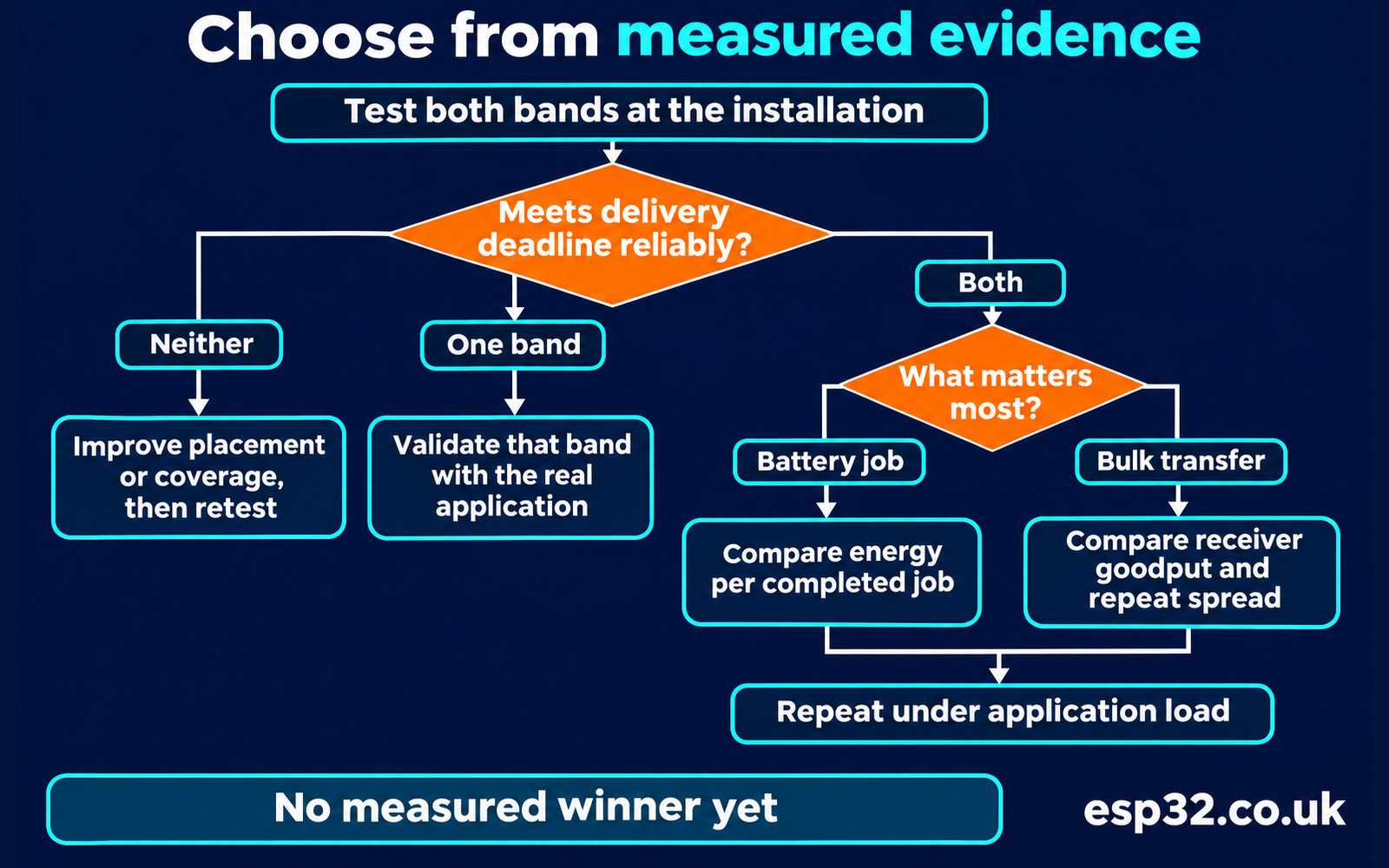
If the measurements are close, consider whether the difference exceeds the spread between repeats. Run another session at a different time before making a strong claim. Avoid turning a modest change on one router into a recommendation for every C5 installation. A second access point or another board provides useful follow-up evidence, but keep those datasets separate.
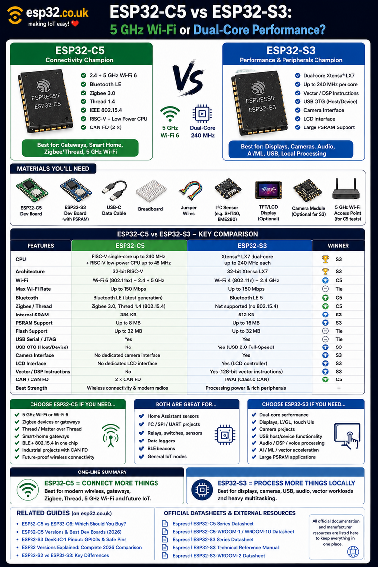
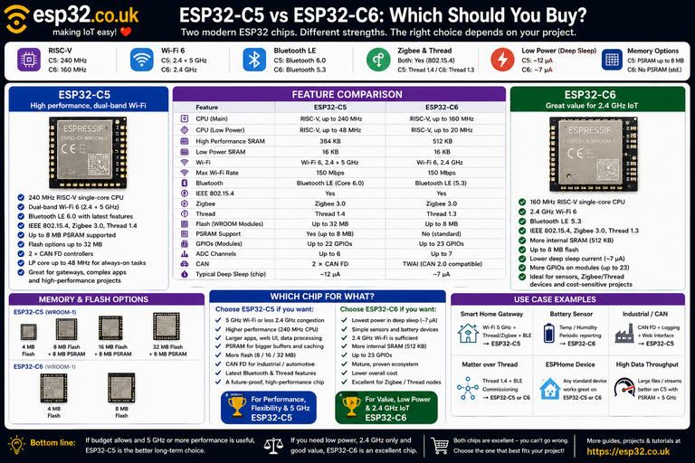
For a broader purchase decision, use the ESP32-C5 versus ESP32-C6 comparison or the C5 versus S3 comparison. This guide answers the narrower question of how one C5 installation behaves on its two available bands. It does not establish the relative processing performance of different chips.
Publish a result readers can reproduce
When measurements become available, add the board revision and antenna, SDK and dependency versions, access point settings, test positions, power boundary and raw-log references beside the results. Describe the workload and number of attempts before announcing a winner. If a metric was unavailable, retain that limitation rather than filling the gap with a specification.
Keep the conclusion local to the evidence: the selected configuration met a stated requirement at named positions, under recorded conditions. Until those readings exist, this article remains a test guide with blank results tables. The next useful step is to run the same procedure on both bands and let completed jobs, receiver measurements and energy records determine the recommendation.